Staring at a matrix equation like Ax = b can feel a little intimidating, but your goal is always the same: find that unknown vector 'x'. To get there, you've got a few solid tools in your belt. The most common are Gaussian elimination, using the matrix inverse, and applying Cramer's Rule. Think of them as different tools for different jobs—each one is perfect for a specific kind of problem.

Your Starting Point for Solving Matrix Equations

Before you jump into the number-crunching, take a moment to pick the right strategy. This one decision can save you a ton of time and headache. The best approach really depends on the size of your matrix, whether it has special properties (like being square), and what you're trying to find.

Some methods are great shortcuts for small, simple systems. Others are more powerful and can handle just about anything you throw at them. We'll focus on the three foundational techniques that are the bread and butter of linear algebra. These aren't just abstract theories; they're the practical tools you'll use to solve real problems.

• Gaussian Elimination: This is your reliable, all-purpose workhorse. It's a systematic process of simplifying the equation until the solution practically falls into your lap. Crucially, it's the only method that works for non-square or singular matrices.
• The Matrix Inverse: Think of this as the elegant shortcut. If you have a square, non-singular matrix, you can find its inverse (A⁻¹) and solve for 'x' with one clean multiplication: x = A⁻¹b.
• Cramer's Rule: This is a formula-based method that's fantastic for small 2x2 or 3x3 systems. It's especially handy when you only need to find the value of a single variable and don't want to solve the whole system.

A Glimpse into the History of Matrix Math

It's pretty amazing to think that the core ideas we use today have ancient roots. The ancient Chinese developed one of the earliest systematic methods for solving these kinds of equations over 2,000 years ago. Around 200 BC, a text called 'Nine Chapters of Mathematical Art' described a technique of arranging coefficients on a counting board and performing operations that we'd now recognize as Gaussian Elimination. To learn more, Harvard's historical overview offers a fascinating look into these early methods.

Key Takeaway: The "best" way to solve a matrix equation depends entirely on the problem. Gaussian elimination is the most versatile, the inverse method is a fast shortcut for eligible cases, and Cramer's Rule is perfect for quickly finding one variable in a small system.

To help you decide which tool to pull out of your toolbox, here’s a quick comparison.

Comparison of Methods for Solving Matrix Equations

This table breaks down the main methods, helping you choose the most efficient approach for your specific problem.

Method	Best For	Complexity	Key Requirement
Gaussian Elimination	Any system, especially large or non-square ones.	Can be long, but always works.	None. It's universally applicable.
Matrix Inverse	Small, square systems where the inverse is known.	Finding the inverse can be very intensive.	Matrix must be square and invertible.
Cramer's Rule	2x2 or 3x3 systems, especially for one variable.	Calculating determinants gets complex fast.	Matrix must be square and invertible.

Knowing which method to apply is a skill that comes with practice. The more problems you work through, the more you'll develop an intuition for the most direct path to a solution.

If you're looking to sharpen your study habits for math, our guide on how to study math effectively has some great, practical strategies. Getting comfortable with these techniques is a huge step, as they unlock your ability to solve complex problems in engineering, physics, computer graphics, and data science.

Getting Your Hands Dirty with Gaussian Elimination

When you need a surefire method that can handle any matrix, no matter the size or solution type, Gaussian elimination is your workhorse. You might also know it as row reduction. It's easily the most robust and versatile tool in your linear algebra toolkit, systematically breaking down a complicated system into something you can solve in your sleep.

The first move is to combine your coefficient matrix, A, with the constant vector, b. This creates a single, larger matrix called an augmented matrix, which we write as [A|b]. Think of this as setting the stage—once you have the augmented matrix, the real work of simplifying can begin.

The Three Fundamental Row Operations

To wrestle this augmented matrix into a simpler form, you have three legal moves at your disposal. Mastering these elementary row operations is the secret to getting the right answer every time.

• Row Swapping: You can swap any two rows, plain and simple. This is just like reordering the equations in your original system, which has zero effect on the final solution.
• Row Scaling: You can multiply an entire row by any number that isn't zero. This is the matrix equivalent of multiplying both sides of an equation by a constant.
• Row Combining: This is the powerhouse operation. You can add a multiple of one row to another row, which is how you'll strategically create zeros and simplify the matrix.

Your goal here is to use these three operations to get the left-hand side of your augmented matrix into what we call row-echelon form. It looks like a staircase, where the first non-zero number in each row (the "pivot") is to the right of the pivot in the row above it, and everything below each pivot is a zero.

This infographic lays out the common paths to solving a matrix equation, and you'll notice that Gaussian elimination is the foundational technique.

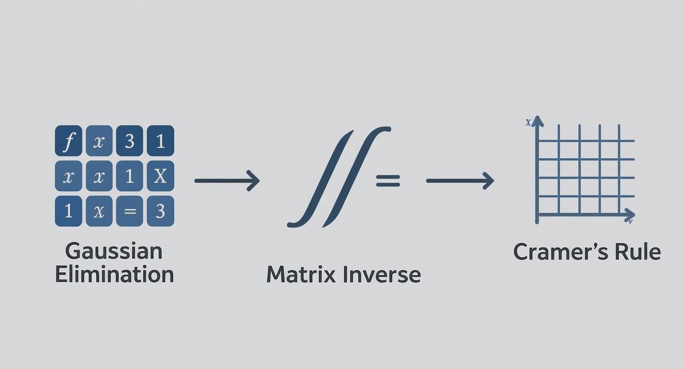
While there are other ways to get to the answer, row operations are the engine that drives the most reliable method.

A 3x3 Example in Action

Let's see this in action with a concrete example. Imagine you're faced with this system of equations:

x + 2y + z = 2
3x + 8y + z = 12
4y + z = 2

First things first, we build the augmented matrix [A|b]:

[ 1 2 1 | 2 ]
[ 3 8 1 | 12 ]
[ 0 4 1 | 2 ]

We want to create zeros below the first pivot (the 1 in the top-left corner). To get rid of that 3 in the second row, we can subtract 3 times the first row from the second row. Our operation is R2 -> R2 - 3*R1.

[ 1 2 1 | 2 ]
[ 0 2 -2 | 6 ]
[ 0 4 1 | 2 ]

Looking good. Now, we want to eliminate the 4 in the third row, using the pivot from the second row. We'll perform the operation R3 -> R3 - 2*R2.

[ 1 2 1 | 2 ]
[ 0 2 -2 | 6 ]
[ 0 0 5 | -10 ]

Perfect. The matrix is now in row-echelon form. The final piece of the puzzle is called back-substitution. We just turn this matrix back into a system of equations, starting from the bottom row and working our way up.

• Row 3 gives us: 5z = -10, which means z = -2.
• Row 2 gives us: 2y - 2z = 6. Plugging in our value for z, we get 2y - 2(-2) = 6, which simplifies to 2y + 4 = 6, so y = 1.
• Row 1 gives us: x + 2y + z = 2. With our known y and z, we have x + 2(1) + (-2) = 2, which means x = 2.

And there it is: the solution is x=2, y=1, and z=-2. This step-by-step process is a core concept in linear algebra, and you can see more examples in our guide on how to solve systems of linear equations.

How to Spot the Special Cases

One of the best things about Gaussian elimination is that it doesn't just fail silently; it tells you exactly when a system has no solution or infinitely many. These weird cases pop up naturally as you perform the row operations.

Pro Tip: As you're reducing the matrix, always watch for a strange-looking row. If you end up with a row like [0 0 0 | c] where c is any number except zero, you've hit a contradiction (like 0 = 5). This means there is no solution. On the other hand, if you get a row of all zeros like [0 0 0 | 0], it signals a dependent system that has infinitely many solutions.

Using the Matrix Inverse for a Direct Solution

Sometimes, grinding through row operations isn't the only way to solve a matrix equation. There's a much more direct route: the matrix inverse. This method offers an elegant, powerful way to solve Ax = b with a single, clean calculation: x = A⁻¹b.

This approach almost feels like a shortcut. Instead of methodically chipping away at an augmented matrix, you find the inverse of the coefficient matrix A, multiply it by the constant vector b, and the solution vector x just pops out. It's incredibly satisfying, but this shortcut comes with a few strict conditions.

When Can You Use the Matrix Inverse?

Unlike the workhorse method of Gaussian elimination, using the inverse isn't a universal tool. It only works if your matrix A checks two specific boxes:

• It has to be a square matrix. This just means it needs the same number of rows and columns (a 2x2, 3x3, etc.).
• It must be non-singular (or invertible). In simple terms, the matrix has to have an inverse. The quickest way to check is by calculating its determinant—if the determinant is not zero, you're good to go.

If your matrix fails either of these tests, you'll have to fall back on another technique like row reduction. But when the conditions are met, the inverse method is a remarkably efficient path to the answer, especially for smaller systems.

Calculating the Inverse of a 2x2 Matrix

For a 2x2 matrix, finding the inverse is a straightforward process with a simple formula. Let's take a general matrix A:

A = [a b]
[c d]

First, you calculate the determinant, which is simply ad - bc. As long as that’s not zero, you can find the inverse A⁻¹ using this formula:

A⁻¹ = (1 / (ad - bc)) * [ d -b]
[ -c a]

Take a close look at what’s happening inside the matrix. The elements on the main diagonal (a and d) swap places, while the other two elements (b and c) just flip their signs. Then, you multiply the whole thing by one over the determinant.

A Worked 2x2 Example

Let's put this into practice with a system of equations:

2x + 4y = 10
1x + 3y = 6

First, we'll write this in matrix form, Ax = b:

[2 4] [x] = [10]
[1 3] [y] [6]

To solve this, we need the inverse of matrix A. Let's start with the determinant: det(A) = (2)(3) - (4)(1) = 6 - 4 = 2. Since the determinant isn't zero, an inverse definitely exists.

Now, we just plug our values into the inverse formula:

A⁻¹ = (1/2) * [ 3 -4]
[ -1 2]

Multiplying the 1/2 into the matrix gives us:

A⁻¹ = [ 1.5 -2]
[ -0.5 1]

With the inverse ready, we can solve for x using our magic formula, x = A⁻¹b:

[x] = [ 1.5 -2] [10]
[y] [-0.5 1] [ 6]

All that's left is to perform the matrix multiplication:

x = (1.5)(10) + (-2)(6) = 15 - 12 = 3
y = (-0.5)(10) + (1)(6) = -5 + 6 = 1

And there it is. The solution is x = 3 and y = 1. It's a much cleaner process than row-reducing the augmented matrix.

Why Not Always Use the Inverse?
While this method is elegant, it's often less efficient for larger matrices (3x3 and up). From a computational standpoint, the number of calculations needed to find the inverse of a large matrix skyrockets. It's actually much faster for a computer to solve the system using Gaussian elimination. That's why software packages almost always default to methods based on row reduction—they're faster and more numerically stable as matrices get bigger.

This trade-off is a key concept. For small systems you're solving by hand, the inverse can be a fantastic time-saver. But for the large-scale problems you'd find in engineering or data analysis, methods like LU decomposition (which is essentially a streamlined version of Gaussian elimination) are the go-to for their superior speed and reliability.

Applying Cramer's Rule to Find Specific Variables

What if you don't need the entire solution vector? Sometimes, an engineering or physics problem only asks for a single variable—maybe you just need to find the current I₃ in a circuit—and solving for everything else is a waste of time. This is where Cramer's Rule really shines. It's a specialized tool that uses determinants to zero in on one variable at a time.

Unlike Gaussian elimination, which is a full-system workout, Cramer's Rule offers a direct formula. It lets you jump straight to the value of x, y, or any other variable you need, as long as the system is square and has a unique solution. I’ve always found it to be a fantastic shortcut for small systems, especially when you're up against the clock on an exam and only need one piece of the puzzle.

The rule itself has a rich history, rooted in the work of mathematicians like Gottfried Leibniz and Carl Friedrich Gauss, who formalized determinant theory. While Leibniz first touched on determinants way back in 1693, it was Gabriel Cramer who, in 1750, published his famous formula, giving us a clean, determinant-based method for solving linear systems. If you're curious, you can explore more about the deep history of matrices and their pioneers.

The Core Idea Behind Cramer's Rule

At its heart, the rule is beautifully simple. The value of any given variable is just a ratio of two determinants.

The denominator is always the determinant of the main coefficient matrix, which we’ll call D. The numerator is the determinant of a slightly altered matrix. To find it, you just take the original coefficient matrix and replace the column corresponding to your target variable with the constants from the b vector.

So, if you want to find x, the formula is x = Dx / D, where Dx is the determinant of matrix A but with its first column swapped out. Need y? No problem. The formula is y = Dy / D, where you swap out the second column. This elegant pattern holds for any variable in the system.

A Practical Walkthrough with a 2x2 System

Let's make this less abstract with a quick 2x2 example. Imagine you have this system:

4x + 2y = 24
2x + 3y = 16

Our coefficient matrix A is [4 2; 2 3], and our constant vector b is [24; 16].

First things first, we need the determinant of the main coefficient matrix, D. This is a critical check—if D is zero, Cramer's Rule is off the table because there isn't a unique solution.

• D = (4)(3) - (2)(2) = 12 - 4 = 8

Since D isn't zero, we're good to go.

Next, let's find x. We need the determinant Dx, which we get by replacing the first column (the x-coefficients) with our b vector.

• The new matrix for Dx is [24 2; 16 3].
• Dx = (24)(3) - (2)(16) = 72 - 32 = 40

Now for y. We do the same thing, but this time we replace the second column (the y-coefficients) with the b vector.

• The new matrix for Dy is [4 24; 2 16].
• Dy = (4)(16) - (24)(2) = 64 - 48 = 16

All that's left is to plug these numbers into our formulas:

• x = Dx / D = 40 / 8 = 5
• y = Dy / D = 16 / 8 = 2

And there it is: the solution is x = 5 and y = 2. It's a very mechanical process, which can make it less prone to the kind of procedural slip-ups that sometimes happen during row reduction.

A Word of Caution: Cramer's Rule is a sprinter, not a marathon runner. It's incredibly fast for 2x2 systems and still manageable for 3x3s. But the computational effort explodes from there. For a 4x4 system, you’d have to calculate five different 4x4 determinants—a brutally tedious and inefficient task to do by hand.

Scaling Up to a 3x3 Example

The logic for a 3x3 system is exactly the same, though the determinant calculations take a bit more work. For a system with variables x, y, and z, the solutions are simply:

• x = Dx / D
• y = Dy / D
• z = Dz / D

Here, Dx, Dy, and Dz are the determinants you get by replacing the first, second, and third columns of the coefficient matrix with the constant vector, respectively. While it's perfectly doable, this is the point where many people (including me) start to lean back toward Gaussian elimination unless a problem specifically asks for Cramer's Rule or you genuinely only need one variable. Its strength is in surgical precision for small problems, not brute-force power for large ones.

Modern and Computational Solving Techniques

While it's crucial to grind through row reduction and matrix inverses by hand to really get the concepts, let's be realistic. In the real world of engineering, data science, or computer graphics, nobody is solving a 50x50 matrix with a pencil and paper. For the large, messy systems you'll actually encounter, we lean on computers.

This is where the theory you’ve learned meets modern, practical application.

One of the most powerful "under the hood" methods is LU Decomposition. The idea is to break down the main matrix A into two much simpler ones: a Lower triangular matrix (L) and an Upper triangular matrix (U). Solving Ax = b then becomes a two-part process: first, you solve Ly = b, and then Ux = y.

Why bother? Because this factorization is incredibly efficient, especially if you have to solve for multiple different b vectors using the same A matrix. You do the heavy lifting of the decomposition just once, then fly through the rest. This technique and others really took off after 1948, giving scientists and engineers the tools to solve problems that were completely out of reach by hand.

Solving Matrix Equations with Python

If you're doing any kind of scientific computing, Python's NumPy library is your best friend. It has a simple, direct function that solves Ax = b for you, handling all the messy calculations behind the scenes. More importantly, it's faster and far more numerically stable than trying to compute a matrix inverse yourself.

Let's take this 3x3 system:

• 2x + y - z = 8
• -3x - y + 2z = -11
• -2x + y + 2z = -3

With NumPy, solving it is almost trivial.

import numpy as np

Define the coefficient matrix A

A = np.array([[2, 1, -1],
[-3, -1, 2],
[-2, 1, 2]])

Define the constant vector b

b = np.array([8, -11, -3])

Solve the equation Ax = b for x

x = np.linalg.solve(A, b)

print(x)

Output: [ 2. 3. -1.]

And just like that, we get our answer: x = 2, y = 3, and z = -1. The np.linalg.solve function is highly optimized and should be your go-to for any practical problem. Understanding how these tools work is a stepping stone to more advanced fields, like those involved in planning artificial intelligence.

Using a Graphing Calculator

You don't need a full-blown programming environment to get help from technology. Most students already have a powerful matrix solver sitting in their backpack. Graphing calculators, like the ubiquitous Texas Instruments TI-84, are perfectly capable of handling these problems.

Pro Tip: Your calculator's matrix solver is your secret weapon for checking your work. After you've sweated through a Gaussian elimination problem on an exam, you can quickly punch it into your calculator to confirm your answer. It's a fantastic way to catch a simple arithmetic mistake before it costs you points.

On a TI-84, the process is straightforward:

• Go into the matrix menu and define matrix [A] with your coefficients.
• Create a second matrix, [B], as a single column with your constants.
• From the home screen, you can calculate the solution by typing [A]⁻¹ * [B].

This gives you the solution vector in seconds. Getting comfortable with these tools is a practical skill that extends beyond just getting the right answer for homework. It builds a foundation for tackling more complex challenges. If you want to explore more problem-solving frameworks, take a look at our guide on how to solve math problems step-by-step.

Common Mistakes to Avoid on Exams

Knowing the theory is half the battle; executing it perfectly under the pressure of an exam is the other half. When it comes to matrix equations, the path to the right answer is filled with little traps. A single slip-up, a tiny arithmetic mistake, can cascade through your entire calculation and lead you far from the correct solution.

The most common culprit I see year after year? Simple calculation errors during Gaussian elimination. You're juggling multiple row operations, and it's shockingly easy to add when you meant to subtract or bungle a multiplication. One small mistake in the first few steps can completely derail your work, costing you points and precious time.

Another classic pitfall is messing up a 3x3 determinant. With all the multiplications and subtractions involved, it's incredibly easy to get a sign wrong. This is a critical error, especially if you're banking on Cramer's Rule, where your entire solution is built on a foundation of correctly calculated determinants.

Forgetting the Rules of Matrix Multiplication

A more fundamental mistake I often see is when students treat matrices like regular numbers. You absolutely have to remember that matrix multiplication is not commutative. The order is everything.

When you're using the inverse method, the formula is always x = A⁻¹b. A surprisingly common error is to flip the order and calculate bA⁻¹. Not only will this almost certainly give you the wrong answer, but a lot of the time, the dimensions won't even allow for that multiplication to happen.

Exam Day Tip: Before you multiply two matrices, take two seconds to jot down their dimensions next to each other, like (3x3) next to a (3x1). If those inner numbers don't match, you know you can't multiply them. This simple sanity check can stop you from heading down a dead-end street.

Strategic Test-Taking Habits

Beyond just avoiding calculation mistakes, your strategy for tackling the problem itself can make a world of difference. Don't just jump in with the first method that pops into your head. Pause for a moment and think about the most efficient path forward.

Here are a few practical habits to build for exam day:

• Choose Your Method Wisely: If a question only asks for the value of one variable in a simple 2x2 system, Cramer's Rule is probably your fastest route. For bigger systems or non-square matrices, go straight to Gaussian elimination. It's the most reliable workhorse.
• Recognize the Zero Determinant: The second you calculate a determinant and get zero, stop. This is a massive clue. It tells you there isn't a unique solution, so you can't use the inverse method or Cramer's Rule. Make a note that the determinant is zero, then switch gears to row reduction to figure out if there are no solutions or infinitely many.
• Use Your Calculator as a Guardrail: If you’re allowed a calculator, use it to double-check your work, not just do it for you. After you've found an inverse or a determinant by hand, a quick verification on your calculator can give you the confidence that you're on the right track before you sink more time into the problem. It’s the smartest way to catch those pesky little errors.

Frequently Asked Questions

When you're first diving into matrix equations, a few common questions always pop up. Getting these concepts straight is often the key to moving forward with confidence.

What Happens if the Determinant Is Zero?

This is a big one. If you calculate the determinant of your coefficient matrix A and it comes out to zero, you've hit a critical point. The matrix is called singular, and this immediately tells you it doesn't have an inverse.

So, right off the bat, you know the matrix inverse method (x = A⁻¹b) is off the table. A zero determinant means you're looking at one of two possibilities for your system of equations:

• No solution exists at all. The equations are inconsistent.
• There are infinitely many solutions. The system is dependent.

To figure out which scenario you're dealing with, your best bet is to go back to Gaussian elimination. Row-reducing the augmented matrix will give you the answer. If you end up with a nonsensical row like [0 0 0 | 5], it’s a clear sign there's no solution. On the other hand, a row of all zeros, like [0 0 0 | 0], points to infinite solutions.

Which Solving Method Is the Best?

Honestly, there's no single "best" method. The right tool really depends on the job at hand.

Think of Gaussian elimination as your all-purpose wrench. It's the most powerful and versatile technique because it works on any size system (n x m) and can handle any outcome—unique, no solution, or infinite solutions. It's your reliable fallback.

The Matrix Inverse method is super efficient, but only for small, square systems (like a 2x2 or 3x3) and only when the matrix is non-singular. Likewise, Cramer's Rule can be a neat shortcut if you only need to find the value of a single variable in a small system, but it gets wildly complicated for anything bigger than a 3x3.

When you get to the massive systems used in fields like engineering or data science, nobody does it by hand. They use computational methods like LU Decomposition or lean on powerful software libraries in Python or MATLAB that are built to crunch the numbers.

Can a Calculator Solve All Matrix Equations?

For the most part, yes. A good graphing calculator, like a TI-84, can find determinants, compute inverses, and even solve systems of equations for you. They are invaluable for checking your work or when you're dealing with messy numbers where a manual slip-up is likely.

But here’s the reality check: on an exam, you'll almost certainly be asked to show your work. Your professor wants to see that you understand the underlying process, not just that you know which buttons to press.

My advice? Master the manual methods first. Use your calculator as a powerful tool to verify your answers, not as a crutch to avoid learning the concepts.

---

Struggling with a tricky problem set? Feen AI can provide step-by-step explanations for your exact math, physics, or chemistry questions. Upload a photo of your assignment and get clear, instant help.