How to solve systems of linear equations: A Complete Guide

At its core, solving a system of linear equations is about finding a point of agreement. You're looking for the specific values for your variables that make every single equation in the system true at the same time. The most common paths to get there are graphing, substitution, and elimination, with each offering a different angle to find where the lines cross.

What Are Systems of Linear Equations Anyway?

It’s easy to get lost in the algebra, but try to think of a system of linear equations as a set of rules or conditions for a real-world problem. Each equation is a constraint, and the "solution" is that sweet spot where every rule is satisfied simultaneously.

For example, imagine a small business trying to find its break-even point. One equation could model total costs (your fixed overhead plus what it costs to make each item), while another represents total revenue (the price per item times how many you sell). The solution—the point where those two lines intersect—tells you exactly how many units you need to sell to cover your costs perfectly.

The Core Components of a System

Every linear equation is built from the same basic parts. Getting familiar with them makes the whole process feel much less abstract.

• Variables: These are the unknowns you're hunting for, usually written as x and y. They can stand for anything from the number of products sold to the speed of a train.
• Coefficients: These are the numbers that multiply the variables. In 2x + 3y = 7, the numbers 2 and 3 are the coefficients.
• Constants: These are the fixed numbers that stand on their own, like the 7 in our example. They represent a known value or condition.

The idea of systematically solving these problems is far from new. Early methods can be traced back more than 2,000 years to the ancient Chinese text The Nine Chapters on the Mathematical Art. This classic work laid out procedures for solving systems using counting rods to represent coefficients and constants.

Visualizing the Possible Outcomes

When you start working on a system, you’ll quickly find there are only three possible outcomes. Each one reveals something different about how the equations relate to each other.

A solution to a system of linear equations is the point—or set of points—where all the individual lines (or planes in higher dimensions) intersect. It's the common ground where every equation's rules are simultaneously true.

The image above gives a great picture of what this looks like in three dimensions. While pairs of planes intersect to form lines, there's no single point that lies on all three. This is a classic example of an inconsistent system with no solution.

For more deep dives into advanced math topics and helpful tutorials, you can always explore the articles on the Feen AI blog.

See the Solution: Solving Systems by Graphing

Sometimes, the best way to get a feel for a math problem is to literally draw it out. The graphical method does just that—it turns a couple of abstract equations into lines on a graph. The solution you're looking for? It's simply the spot where those two lines cross.

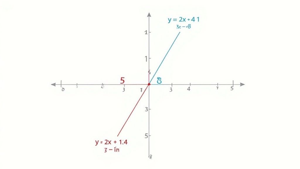
This visual approach is fantastic, especially when you're just starting out. It gives you a concrete picture of what a "solution" really is before you dive into the more algebraic methods. It’s about building intuition first.

Getting Your Equations Ready to Graph

Before you can put pencil to paper (or cursor to screen), your equations need to be in a format that’s easy to plot. The go-to format for this is the slope-intercept form, y = mx + b. It’s a classic for a reason.

Here’s a quick refresher on what the letters mean:

• m is the line’s slope. Think of it as the "rise over run"—how much the line goes up or down for every step it takes to the right.
• b is the y-intercept. This is your starting point, the exact spot where the line crosses the vertical y-axis.

So, if you get an equation like 2x + y = 5, you'll want to get the y by itself. Just subtract 2x from both sides, and you have y = -2x + 5. Now you know exactly what to do: start at 5 on the y-axis, then use the slope of -2 (down two, right one) to find your next point.

What the Intersection Tells You

With both lines drawn on the same coordinate plane, the answer is staring you right in the face. The point where they intersect, written as (x, y), is the one and only combination of x and y that makes both of your original equations true.

But what if the lines don't cross neatly at one point? Graphing is great at revealing these special cases, too.

1. No Solution: The lines are parallel. They have the same slope, so they travel in the same direction forever without ever touching. This means there's no (x, y) pair in the universe that can satisfy both equations. You'll hear this called an "inconsistent" system.

2. Infinite Solutions: You graph both equations and... they're the exact same line. One equation is just a disguised version of the other. In this case, every single point on that line is a valid solution. This is a "dependent" system.

The real power of the graphical method is the immediate visual gut-check it provides. You can see right away if you should be looking for one solution, no solution, or an infinite number of them. That's a huge advantage, even when you plan to use another method to find the exact answer.

Seeing a problem from multiple angles is a cornerstone of modern math education. This idea of connecting the graphical and the algebraic is a well-established teaching practice that helps build a much deeper, more flexible understanding of the concepts. You can explore more about the evolution of these teaching methods/) and why they are so effective.

Using Substitution and Elimination for Exact Answers

While graphing is a great way to see what's going on visually, it isn't always precise. When you need the exact coordinates where two lines cross—not just a good guess—it’s time to roll up your sleeves and use algebra. The two workhorses for this are substitution and elimination.

These methods will give you a clean, precise answer every time. The trick is learning to spot which one is the right tool for the job. Often, the way the equations are set up will give you a clear hint. One method might be a straight shot to the answer, while the other might have you wrestling with messy fractions.

The Substitution Method: When a Variable Is Easy to Isolate

Think of the substitution method as using one equation to unlock the other. It's the perfect strategy when one of your equations already has a variable by itself (like y = 2x - 1) or can be easily rearranged to get it there. You just solve for one variable and then "substitute" that expression into the other equation.

Let’s look at a common real-world scenario: comparing two phone plans.

• Plan A: A flat $20 per month plus $0.10 per gigabyte of data.
• Plan B: A flat $30 per month plus $0.05 per gigabyte of data.

We want to find the exact point where both plans cost the same. Let c be the total cost and g be the gigabytes used. This gives us our system:

1. c = 0.10g + 20
2. c = 0.05g + 30

Since both equations are already solved for c, this is a textbook case for the substitution method.

A Worked Example of Substitution

We can take the expression for c from the first equation and plug it right into the second one. This move is the key—it combines both rules into a single equation with only one variable, g.

0.10g + 20 = 0.05g + 30

Now, it’s just a standard algebra problem. Let's get the g terms on one side and the numbers on the other.

Start by subtracting 0.05g from both sides: 0.05g + 20 = 30

Next, subtract 20 from both sides: 0.05g = 10

Finally, divide by 0.05 to get g by itself: g = 200

So, the plans cost the same when you use 200 gigabytes of data. But we’re not quite done. We still need to find the actual cost. To do that, plug g = 200 back into either of the original equations. Let's use the first one:

c = 0.10(200) + 20 c = 20 + 20 c = 40

The solution is (200, 40). This tells us that at 200 gigabytes of data, both plans will cost exactly $40.

The most common mistake people make with substitution is stopping after finding the first variable. Always plug your answer back into an original equation to find the complete coordinate pair.

The Elimination Method: For Neatly Aligned Equations

What happens when neither variable is easy to isolate? That’s where the elimination method comes in handy. This technique is perfect when the variables in both equations are all lined up in columns. The whole point is to add or subtract the two equations from each other to make one of the variables completely disappear.

Sometimes you get lucky and the coefficients are already opposites (like 3y and -3y). But more often, you’ll have to multiply one or both equations by a constant to create those opposites. As long as you multiply every single term in the equation, you're not changing its value. It might feel like an extra step, but for more complex systems, it's often much faster and cleaner than substitution. The logic here is similar to what you'd use in other algebraic problems—for instance, you can learn more about solving logarithmic equations in our other guides.

A Worked Example of Elimination

Let's imagine a bakery sells two kinds of pastry boxes.

• A box with 3 donuts and 2 muffins costs $12.
• A box with 4 donuts and 4 muffins costs $20.

If we let d be the cost of a donut and m be the cost of a muffin, we can set up our system:

1. 3d + 2m = 12
2. 4d + 4m = 20

Look closely at the coefficients for m. We have a 2m and a 4m. This is a dead giveaway that elimination is a good choice. If we multiply the entire first equation by -2, the 2m will become -4m, which is the perfect opposite of the 4m in the second equation.

Let’s do it: -2(3d + 2m = 12) → -6d - 4m = -24

Now we can just add this modified equation to our second original equation: (-6d - 4m) + (4d + 4m) = -24 + 20 -2d = -4

Just like that, the m terms have been eliminated! Solving for d is now a piece of cake: d = 2

So, each donut costs $2. To find the muffin cost, just plug d = 2 back into either of the original equations. We'll use the first one:

3(2) + 2m = 12 6 + 2m = 12 2m = 6 m = 3

Each muffin costs $3. Our final solution is (2, 3), representing the price of one donut and one muffin.

What Happens When You Have More Than Two Variables? Enter the Matrix.

When you're dealing with just two variables, methods like substitution and elimination work great. But what happens when a third, fourth, or even fifth variable enters the picture? Suddenly, your neat algebraic steps can spiral into a tangled mess of bookkeeping. It's incredibly easy to make a small error that throws the whole solution off.

This is exactly where matrices come to the rescue. They provide a clean, organized, and surprisingly powerful way to handle these bigger, more complex problems.

A matrix is just a rectangular grid of numbers. Think of it as a simple container that holds all the coefficients and constants from your system of equations. By stripping away the variables (x, y, z, etc.), we can focus purely on the numbers, making the calculations much, much tidier.

This infographic gives a great overview of the different algebraic methods and how they all connect.

Notice that regardless of the path you take—substitution, elimination, or the matrix methods we're about to cover—the final step is always the same: checking your answer. It’s a non-negotiable part of the process.

First Things First: Setting Up the Augmented Matrix

Your first move is to translate the system of equations into what's called an augmented matrix. It sounds technical, but it’s actually very intuitive. You’re just creating a grid with the coefficients of your variables, then "augmenting" it with one more column for the constants—the numbers on the other side of the equals sign. We usually draw a vertical line to keep them separate.

Let’s take this three-variable system as an example:

• x + 2y - z = 4
• 2x - y + 3z = 7
• 3x + y + 2z = 1

To turn this into an augmented matrix, you just pluck out the numbers. The key is to keep them lined up in their original columns for x, y, and z:

[ 1 2 -1 | 4 ] [ 2 -1 3 | 7 ] [ 3 1 2 | 1 ] That's it. Each row still represents an equation, but now your system is organized and ready for the real work to begin.

The Game Plan: Simplifying with Gaussian Elimination

From here, our main strategy is Gaussian Elimination. This is just a systematic process for simplifying the matrix until the solution is staring you right in the face. The goal is to transform the matrix into row-echelon form, which basically means getting a triangle of zeros in the bottom-left corner.

To do this, you have three simple but powerful moves at your disposal, called elementary row operations:

• Swap two rows. This is like just reordering your list of equations. No harm done.
• Multiply a row by any non-zero number. This is the same as multiplying both sides of an equation by a constant.
• Add a multiple of one row to another row. Here's the magic. This is the matrix version of the elimination method you already know, where you combine equations to cancel out a variable.

The whole point is to strategically use these operations to create zeros. Looking at our example matrix, a good first step would be to get rid of the 2 in the second row and the 3 in the third row. To do that, we could add -2 times the first row to the second row, and then add -3 times the first row to the third.

Gaussian Elimination isn't a magic trick. It's a reliable, step-by-step process that will simplify any system of equations, no matter how big it gets. It always works.

The Payoff: Finding the Solution with Back-Substitution

Once you’ve used row operations to get your matrix into that nice row-echelon form, the heavy lifting is done. Your simplified matrix might look something like this (note: these aren't the exact results from our example):

[ 1 2 -1 | 4 ] [ 0 -5 5 |-1 ] [ 0 0 -2 |-6 ] Now, all you have to do is translate this back into equations:

• x + 2y - z = 4
• -5y + 5z = -1
• -2z = -6

Look at that last equation! It immediately tells you that -2z = -6, which means z = 3. You've found your first variable. From here, a domino effect called back-substitution kicks in. You take the value for z you just found and plug it into the middle equation to solve for y. Then, with y and z in hand, you plug them both into the top equation to find x. It’s a clean cascade that reveals the final solution one variable at a time.

A Different Path: Cramer's Rule

While Gaussian Elimination is the go-to workhorse for matrix problems, there's another technique worth knowing: Cramer's Rule. This method takes a completely different approach, using something called determinants—a special number you can calculate from a square matrix—to solve for each variable directly.

Cramer's Rule can be a real time-saver for smaller systems (like 2x2 or 3x3), especially if you only need to find the value of a single variable instead of the whole set. But be warned: for larger systems, the calculations needed to find all the determinants grow exponentially. In those cases, sticking with Gaussian Elimination is almost always the more practical and efficient choice.

Handling No Solution and Infinite Solution Cases

Not every system of equations ties up with a neat (x, y) solution. Sometimes, the equations you’re working with lead to a dead end where there’s no answer at all, or they open up to an endless number of them. Knowing how to spot these special cases is just as important as finding a standard solution.

These situations aren't errors; they actually reveal something important about the relationship between the equations. They're either working against each other (no solution) or basically saying the same thing in two different ways (infinite solutions). Learning the algebraic red flags for each is key to mastering these problems.

Identifying an Inconsistent System with No Solution

You’ll know you’ve hit an inconsistent system when your algebra leads you to a statement that is just plain false. It's a clear signal that the lines represented by your equations are parallel and, as we know, parallel lines never intersect.

Imagine you're solving this system with the elimination method:

• x - 2y = 5
• -2x + 4y = 8

Your first instinct might be to multiply the first equation by 2 to get the x terms to cancel out.

Doing that gives you 2x - 4y = 10.

Now, when you add this to the second equation, something odd happens: (2x - 4y) + (-2x + 4y) = 10 + 8

Both the x and y terms completely vanish, leaving you with: 0 = 18

This statement is impossible. It’s an algebraic contradiction, and it’s your definitive proof that the system has no solution.

Pro Tip: Don't second-guess your work when you see a result like 0 = 18 or 5 = -3. A false statement is a valid, definitive outcome—it simply means there is no coordinate pair on the planet that can make both equations true.

Uncovering a Dependent System with Infinite Solutions

The other special case pops up when your equations are essentially duplicates of each other, just in disguise. This is what we call a dependent system, and it means both equations describe the exact same line. Naturally, every single point on that line is a solution.

The algebraic signal for this is a statement that is always true, no matter what.

Take a look at this system:

• 3x + y = 7
• 6x + 2y = 14

If we multiply the first equation by -2 to set up elimination, we get: -6x - 2y = -14

Adding this to the second equation results in a total wipeout on both sides of the equals sign: (-6x - 2y) + (6x + 2y) = -14 + 14 0 = 0

This is a universally true statement. It tells you that the two original equations weren't independent at all; one was just a multiple of the other. Therefore, the system has infinite solutions.

The Most Important Habit: Verifying Your Answer

Whether you find one solution, none, or an infinite number of them, your final step should always be verification. For a unique solution like (2, 3), this is easy—just plug the values back into both original equations to make sure they hold true. It’s a quick check that can save you from simple but costly mistakes.

For these special cases, verification looks a bit different:

• No Solution: Go back and double-check the arithmetic that led to your false statement (like 0 = 18). A small calculation error can sometimes trick you into thinking there's no solution when there is one.
• Infinite Solutions: Check if one equation is a direct multiple of the other. With 3x + y = 7 and 6x + 2y = 14, you can quickly see the second equation is just the first one multiplied by two. This confirms they're the same line.

Making verification a non-negotiable habit builds both confidence and accuracy. And for those really tricky problems, you can always use a tool like Feen AI to scan your work and get a second opinion on your solution.

Common Questions About Linear Equations

As you get the hang of solving systems of linear equations, you'll find a few questions pop up again and again. I've been there. This section is your go-to guide for those common sticking points, designed to clear up confusion and help you pick the right tool for the job.

Getting clear on these details is what builds real confidence. It’s the difference between just memorizing steps and truly understanding why you're choosing one method over another, which is crucial when you move on to more complex problems.

When Should I Use Substitution Instead of Elimination?

This is easily the most common question I get, and the good news is the equations themselves usually give you a hint. The key is to look at the structure of the system before you dive in.

Go for the substitution method when:

• One equation is already solved for a variable, like y = 2x - 1. This is a huge green light. Half the work is already done for you, so just plug it in.
• A variable has a coefficient of 1 or -1 (think x + 3y = 9). Isolating that x is clean and simple, and you won’t have to deal with messy fractions.

On the other hand, the elimination method is your best friend when:

• The coefficients for one variable are perfect opposites, like a 3x in one equation and a -3x in the other. Just add the two equations together, and poof—that variable disappears.
• No variable is easy to isolate, but you can see a simple path to create opposite coefficients by multiplying one or both equations by a small number.

The goal is always to find the path of least resistance. Choosing the right method from the start saves a ton of time and, more importantly, dramatically reduces your chances of making a small calculation error that throws everything off.

Can You Solve a Three-Variable System by Graphing?

Technically, yes. Practically? No, not by hand. It’s a bit of a nightmare. A two-variable system gives you lines on a flat 2D plane, which is easy enough to sketch. But a three-variable system represents planes floating in 3D space.

To find the solution, you'd have to pinpoint the exact spot where three different planes intersect. Just trying to visualize that is tough, let alone drawing it accurately enough on paper to find a precise (x, y, z) coordinate. This is exactly why we rely on algebraic methods like Gaussian elimination for systems with three or more variables. They’re built for that kind of precision.

What Does "Infinite Solutions" Mean in the Real World?

Getting "infinite solutions" as an answer feels abstract and a little weird. How can a real-world problem have endless answers? It almost always means you have redundant information—two of your equations are secretly describing the same relationship. One is just a disguised version of the other.

Imagine a simple business scenario where a vendor is comparing T-shirt suppliers:

• Supplier A charges a $50 setup fee plus $10 per shirt.
• Supplier B charges a $100 setup fee plus $20 for every two shirts.

They look different at first, right? But Supplier B's deal is still just $10 per shirt, making it a consistently worse deal due to the higher fee. However, if their setup fees were identical, their cost models would be the exact same line. That’s your "infinite solutions" scenario. It’s a signal that two pieces of your data aren't independent.

For students juggling assignments, finding efficient ways to manage your workload is a similar puzzle. You might find some practical tips in our guide on how to write an essay fast.

---

Stuck on a tricky math problem or just want to check your work? With Feen AI, you can snap a photo of your assignment and get instant, step-by-step explanations for everything from algebra to calculus. Stop guessing and start understanding. Try it today at https://feen.ai.