How to Solve Differential Equations A Practical Guide

Solving any differential equation comes down to one thing: correctly identifying what kind of equation you're looking at. Once you know if it's separable, linear, exact, or something else, you can apply a specific, time-tested method to crack it. The entire game is about first classifying the equation and then executing the right playbook.

Your Roadmap to Solving Differential Equations

Staring at a differential equation and not sure where to begin? You're in the right spot. Think of this guide as your practical roadmap. We're skipping the dense, abstract theory and focusing on the hands-on methods that actually lead to a solution. I'll walk you through how to quickly size up your equation and pair it with the most efficient technique.

This isn't just some modern academic drill; it's a process that's been sharpened over centuries. Differential equations first showed up in the 17th century as a way to tackle real-world physics problems. Pioneers like Isaac Newton and Gottfried Leibniz laid the foundation, and by the 18th century, mathematicians like Euler and Lagrange had built that into a systematic toolkit for modeling everything from planetary motion to simple mechanics. The methods we use today, whether in a textbook or with a tool like Feen AI, are direct descendants of their work. For a deep dive, check out Cajori's historical overview on the topic.

The Core Problem-Solving Workflow

At its heart, the process is a simple decision tree. You look at the equation, figure out its order and form, match that form to a known solution method, and then you just work the steps.

This flowchart lays out the entire workflow, from that first look at the equation all the way to the final solution.

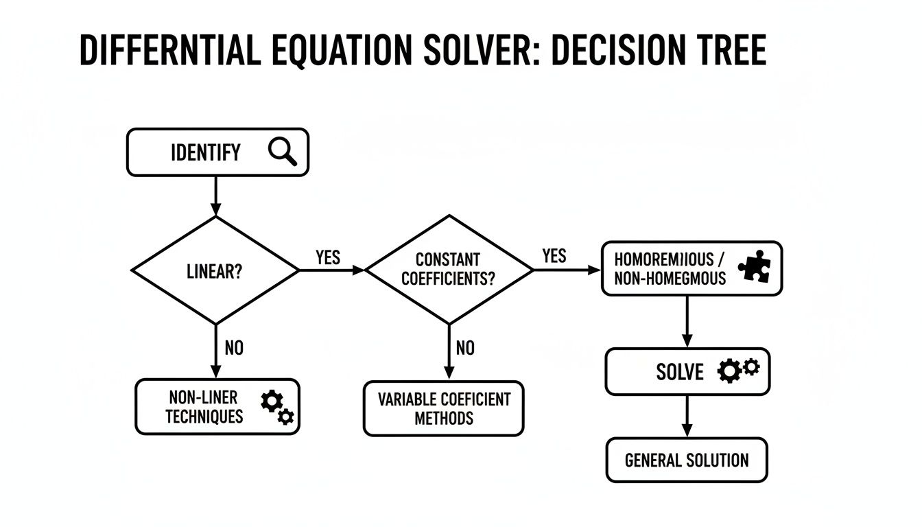
As you can see, everything hinges on that initial diagnosis. If you pick the wrong path from the start, you’ll just hit a dead end.

To help you make that first choice quickly, here’s a handy reference table.

Quick Guide to Choosing Your Solution Method

This table provides a quick reference for matching common differential equation types with the correct solution method, helping you get started faster.

Equation Type	Key Feature	Common Method
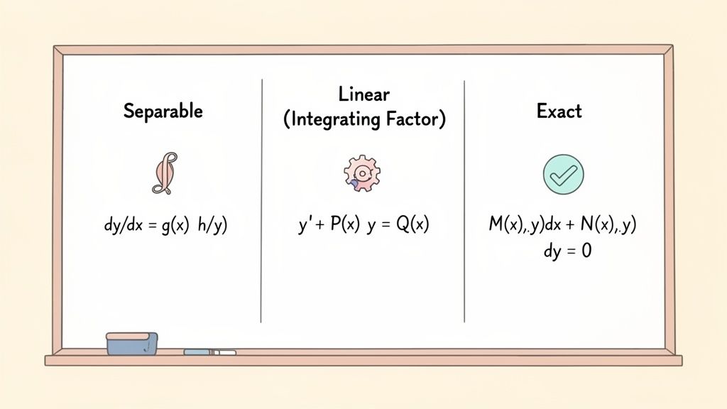
Separable	Can be written as f(y)dy = g(x)dx	Separation of Variables
First-Order Linear	Form: y' + P(x)y = Q(x)	Integrating Factor
Exact	Form: M(x,y)dx + N(x,y)dy = 0 where ∂M/∂y = ∂N/∂x	Direct Integration
Second-Order Homogeneous	Form: ay'' + by' + cy = 0	Characteristic Equation
Second-Order Nonhomogeneous	Form: ay'' + by' + cy = g(x)	Undetermined Coefficients or Variation of Parameters

Think of this table as your cheat sheet. When you see an equation, try to match its structure to one of these types, and you'll know exactly which tool to pull out of your toolbox.

A strong grasp of the fundamentals is non-negotiable. If you're feeling rusty on derivatives and integrals, it's wise to review those concepts first, as they are the building blocks for every method we'll cover.

Before you jump into the specific techniques, make sure your calculus skills are sharp. If you need a refresher, our guide on how to understand calculus can help bring you back up to speed. A little prep work now will make the next steps feel a whole lot easier.

Getting a Grip on First-Order Differential Equations

If you're just starting your journey with differential equations, first-order equations are the right place to begin. They're the bedrock for everything that comes later and pop up constantly in fields like engineering and physics. Once you get a solid handle on the main techniques here, you'll build the intuition needed to take on much tougher problems.

First-order equations are defined by having only the first derivative—you'll see a dy/dx or y', but nothing higher. We're going to walk through the three most common types you'll run into and the specific game plan for solving each. Think of these as the essential tools for your mathematical workshop.

The First Move: Separable Equations

The most straightforward type to solve is the separable equation. The name itself tells you the entire strategy: your goal is to get all the y terms on one side with dy and all the x terms on the other side with dx. A little algebraic shuffling is all it usually takes.

Once you've managed that, the equation should look something like f(y)dy = g(x)dx. From there, the path is clear—just integrate both sides. This simple step turns your differential equation into a standard algebraic one, which you can then solve for y.

Let’s look at a classic real-world example. The logistic growth model, which describes how a population grows when resources are limited, is a perfect case of a separable differential equation.

Example: Modeling Population Growth
Imagine a population P changing over time t, governed by this equation:
dP/dt = kP(1 - P/M)

Here, k is the growth rate constant and M is the environment's carrying capacity. To solve this, you separate the variables:
dP / (P(1 - P/M)) = k dt

Integrating both sides (you'll need partial fraction decomposition for the left side) gives you the famous logistic function, a cornerstone of ecological modeling.

Taming Linear Equations with an Integrating Factor

Next up, we have first-order linear equations. These are pretty easy to spot because they fit a standard form:
y' + P(x)y = Q(x)

In this form, P(x) and Q(x) are just functions of x. You can't separate the variables here. Instead, we have to pull a clever trick out of our hats using something called an integrating factor, which we'll call I(x).

The whole point of this integrating factor is to multiply the entire equation by it. When you do, the left side magically transforms into the result of a product rule derivative, which makes it incredibly simple to integrate.

The formula for the integrating factor is always the same:
I(x) = e^(∫P(x)dx)

Once you calculate I(x), you multiply it through the entire equation. The left side will always condense down to d/dx [I(x)y]. Then, it's just a matter of integrating both sides and solving for y.

Example: A Look Inside RC Circuits
A simple resistor-capacitor (RC) circuit in electronics is a perfect application. The equation for the charge q on the capacitor over time t is:
R(dq/dt) + (1/C)q = V(t)

If you divide by R, it clicks right into our standard linear form:
dq/dt + (1/RC)q = V(t)/R

Here, P(t) is just the constant 1/RC. The integrating factor becomes I(t) = e^(∫(1/RC)dt) = e^(t/RC). Multiplying the equation by this factor allows you to find the charge q(t), which is critical for analyzing how the circuit behaves.

Getting comfortable with the integrating factor method is a huge milestone. It’s a powerful, methodical approach that turns what looks like a messy calculus problem into a straightforward, step-by-step process.

Spotting and Solving Exact Equations

The last of the big three first-order types is the exact equation. These usually show up in the form:
M(x,y)dx + N(x,y)dy = 0

An equation is called "exact" if it's secretly the total differential of some function f(x,y). Luckily, there's a simple test to check if it is, using partial derivatives.

• First, take the partial derivative of M with respect to y (pretending x is a constant).
• Then, take the partial derivative of N with respect to x (pretending y is a constant).

If ∂M/∂y equals ∂N/∂x, then your equation is exact.

If the test passes, you know a function f(x,y) exists where ∂f/∂x = M and ∂f/∂y = N. Your mission is to find that function. A common way to do this is to integrate M with respect to x and then take the partial derivative of your result with respect to y to figure out any missing pieces.

The final solution is given implicitly as f(x,y) = C, where C is just a constant. This method requires careful bookkeeping, but it's very direct once you've confirmed the equation is exact. It’s a vital technique in fields from thermodynamics to fluid dynamics.

Solving Second-Order Linear Equations

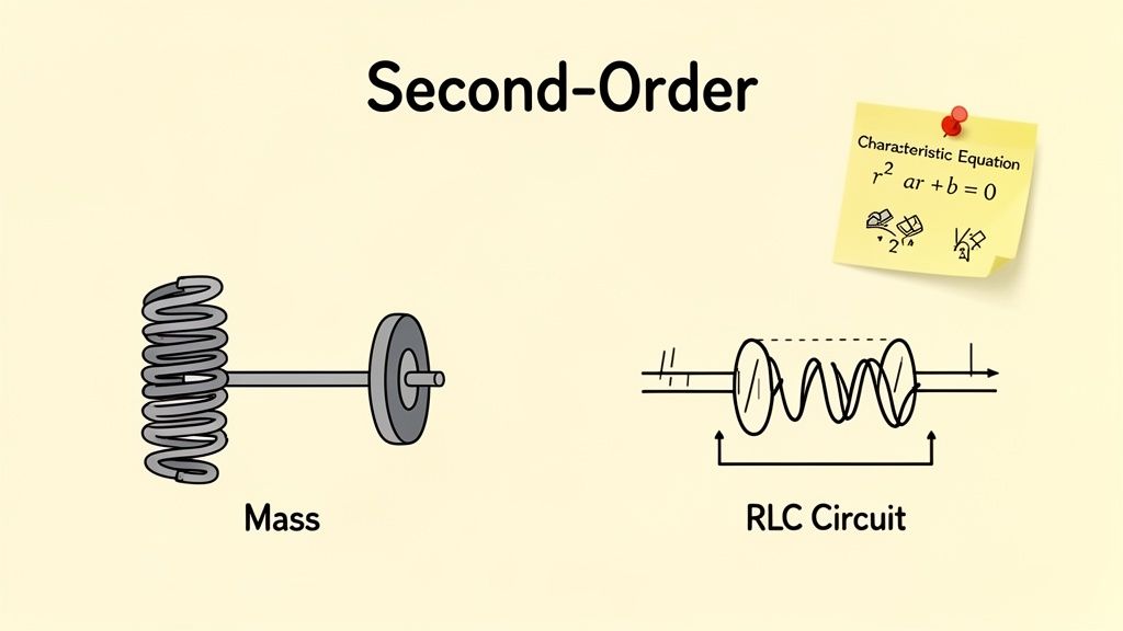
Once you've got a handle on first-order problems, the next big step is tackling second-order linear equations. These are the mathematical workhorses that describe countless physical systems, from the simple sway of a pendulum to the complex oscillations in an RLC circuit. Getting good at these is a major leap in your ability to model the real world.

The standard form you'll see is ay'' + by' + cy = g(x), where a, b, and c are just constant numbers. The function on the right, g(x), is the game-changer; it dictates our entire strategy. Let's break down the two main scenarios you'll run into.

Homogeneous Equations with Constant Coefficients

The most straightforward case is the homogeneous equation, where the right side is simply zero: ay'' + by' + cy = 0. Think of this as describing a system's natural, unforced behavior—like a spring bobbing up and down on its own after you give it a single pull.

To solve it, we make an educated guess that the solution probably looks something like y = e^(rx). Why? Because the derivatives of an exponential are just more exponentials, which gives us a good chance of making them all cancel out to zero.

Plugging this guess into the equation and doing a bit of algebra gets you to the characteristic equation:
ar² + br + c = 0

Suddenly, the calculus problem has turned into a simple quadratic equation. The roots (r) of this equation tell you everything you need to know about the solution. There are three possible outcomes.

• **Case 1: Two Real, Distinct Roots (r₁, r₂) **
  When the discriminant b² - 4ac is positive, you get two different real roots. The general solution is a simple combination of two exponentials: y = C₁e^(r₁x) + C₂e^(r₂x). This typically describes a system that returns to equilibrium without oscillating.

• Case 2: One Real, Repeated Root (r)
  If the discriminant is zero, you've got a single repeated root. The solution needs a small but crucial tweak to make the two parts independent: y = C₁e^(rx) + C₂xe^(rx). That extra x is the secret sauce. This case often represents critical damping, the fastest way to return to equilibrium.

• Case 3: Two Complex Conjugate Roots (α ± βi)
  When the discriminant is negative, you get a pair of complex roots, and this is where oscillation comes in. The solution trades exponentials for sines and cosines: y = e^(αx)(C₁cos(βx) + C₂sin(βx)). The e^(αx) part is the damping (decaying or growing oscillations), and the trig functions are the oscillation itself.

The roots of the characteristic equation aren't just abstract numbers; they are a direct fingerprint of the physical system's behavior. Real roots mean exponential decay or growth. Complex roots mean it's going to oscillate.

Tackling Nonhomogeneous Equations

So, what happens when that right-hand side isn't zero? Now we have a nonhomogeneous equation: ay'' + by' + cy = g(x). That g(x) term represents some kind of external force or input driving the system, like a motor pushing a spring back and forth.

The total solution is always built from two pieces:
y(x) = y_c(x) + y_p(x)

Here, y_c is the complementary solution—you get this by solving the homogeneous version (just set g(x) to zero) exactly as we did above. The new challenge is finding y_p, the particular solution, which is a response to the specific g(x) you're given. We have two main tools for this job.

Method of Undetermined Coefficients

This method is basically a game of "strategic guessing." It's incredibly fast and effective, but only when g(x) is a polynomial, an exponential, a sine or cosine, or some combination of them. The idea is to guess that your particular solution, y_p, has the same general form as g(x).

• If g(x) is something like 3x² + 1, your guess for y_p is Ax² + Bx + C.
• If g(x) is an exponential like 5e^(2x), your guess for y_p is Ae^(2x).
• If g(x) is a trig function like cos(4x), you must include both sine and cosine in your guess: y_p = Acos(4x) + Bsin(4x).

After making your guess, you plug it into the full differential equation and solve for the unknown coefficients (A, B, C, etc.). It’s a fantastic shortcut, but remember, it only works for a handful of function types.

Method of Variation of Parameters

What if g(x) is something messier, like tan(x) or ln(x)? That's when you bring out the big gun: the Method of Variation of Parameters. This is a more powerful, formula-based approach that works for any g(x).

This method starts with the complementary solution you already found, y_c = C₁y₁ + C₂y₂. But instead of constant C's, we "vary the parameters" by turning them into functions, u₁(x) and u₂(x), to find the particular solution:
y_p = u₁(x)y₁ + u₂(x)y₂

Finding u₁ and u₂ requires solving a system of equations that can sometimes lead to some hairy integrals. For more advanced systems, especially in engineering, this step might even require you to solve a system of linear equations. If you find yourself in that spot, having a solid grasp of how to solve matrix equations is incredibly useful, as the techniques overlap directly.

The historical drive to solve these equations wasn't just for academic exercise. In the 1740s, physicists like d’Alembert were wrestling with how to mathematically describe a vibrating guitar string, which led directly to the famous wave equation. A decade later, Euler expanded this to three dimensions, laying the groundwork for modeling everything from sound to light. This 18th-century push to connect math to physical phenomena created the analytical tools still taught in over 90% of university physics and engineering programs today. You can explore the rich history of these ideas in this overview of partial differential equations.

Advanced Techniques for Complex Problems

So far, we’ve tackled methods that work beautifully for problems with a nice, clean structure. But what happens when you’re staring down an equation that just won't fit into those neat boxes? That's when you need to reach deeper into your toolkit for some more powerful strategies.

Sometimes, the smartest way to solve a tough problem is to change the game entirely. We're going to look at two major approaches for these trickier situations: one that transforms the problem into a much simpler world, and another that finds highly accurate approximations when a perfect, exact answer is simply out of reach.

The Power of the Laplace Transform

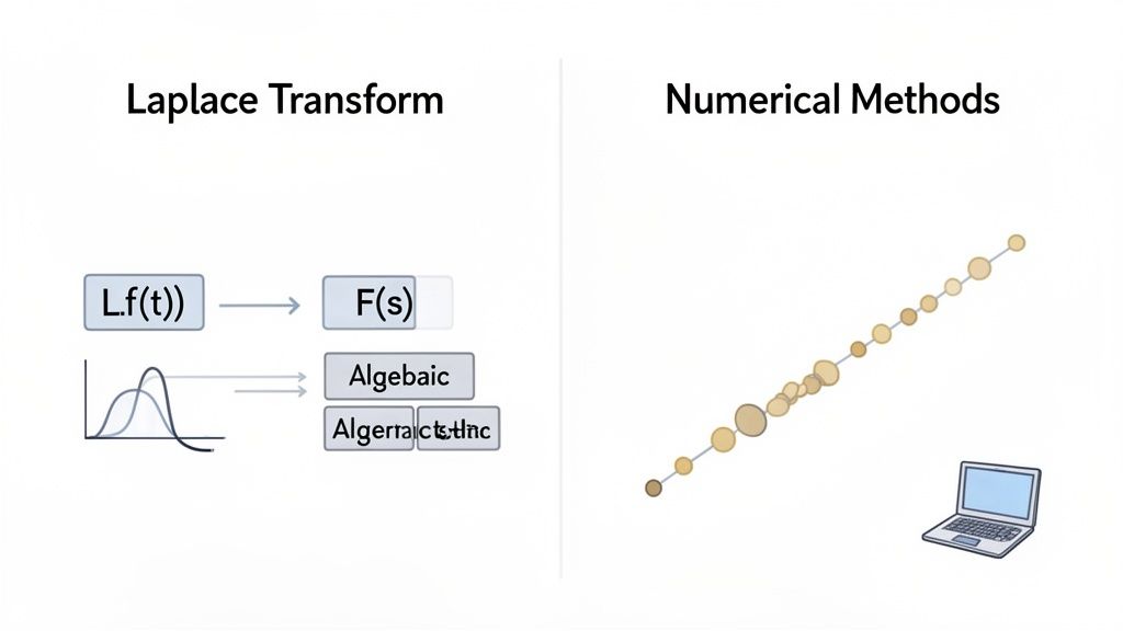
Imagine you could take a gnarly differential equation, wave a magic wand, and turn it into a straightforward algebra problem. That's pretty much what the Laplace Transform does. It’s an incredibly powerful technique, especially common in electrical engineering and control systems, that converts a function of time, f(t), into a function of a complex frequency variable, s, which we call F(s).

Where it really shines is with derivatives. The Laplace Transform turns the calculus operation of differentiation into simple multiplication by s. Suddenly, your entire differential equation—initial conditions and all—becomes an algebraic equation in terms of s that you can just solve.

Here’s the general game plan:

• Transform: Apply the Laplace Transform to both sides of the equation. You'll lean heavily on a standard table of transforms for this.
• Solve: Do the algebra. Rearrange the new equation to solve for Y(s), the transformed version of your solution.
• Inverse Transform: Use an inverse Laplace Transform table to turn Y(s) back into the time domain. What pops out is your final solution, y(t).

This method is an absolute lifesaver for problems with discontinuous functions—think of a switch flipping in a circuit or a motor that suddenly kicks on.

The beauty of the Laplace Transform is how it elegantly handles messy, real-world inputs. It bakes the initial conditions right into the algebraic step, making the whole process incredibly efficient.

When Exact Answers Are Impossible: Numerical Methods

Here’s a hard truth: most differential equations that come from modeling real-world physics and engineering can't be solved with a nice, clean formula. When that happens, we have to let go of finding the perfect answer and instead find a very good approximation. Welcome to the world of numerical methods.

These methods use a computer to build a solution step-by-step. The most basic one, Euler's Method, is the perfect starting point. It’s simple, but it gets the core idea across beautifully.

You start with an initial point (x₀, y₀) and use the differential equation to find the slope of the tangent line there. Then, you take a tiny step h in that direction to guess the next point. You just repeat this process over and over, essentially walking along the solution curve one small step at a time. It might be simple, but it's the conceptual grandfather of the sophisticated solvers you'll find in software like MATLAB and Python libraries.

This shift in mindset—from chasing perfect formulas to finding practical approximations—has a deep history. By the late 19th century, brilliant minds like Henri Poincaré realized that many critical problems had no explicit solution. He developed a qualitative theory to understand a system's long-term behavior even without a formula. This historic pivot broadened what "solving" an equation even means, leading to the mix of analytical and numerical techniques we rely on today. You can explore more about this journey in the history of differential equations.

Understanding numerical methods is crucial. It shows you what’s happening "under the hood" when you ask a computer to solve a problem, and it provides the practical answers that drive modern science when a symbolic solution just isn’t on the table.

Using Feen AI to Check Your Work and Get Unstuck

We've all been there. You spend an hour wrestling with a differential equation, meticulously working through every step, only to find your final answer doesn't match the one in the back of the book. It’s incredibly frustrating, and often, the culprit is a tiny algebra mistake made on the first line.

This is where a tool like Feen AI becomes your secret weapon. Think of it less as a shortcut and more as a 24/7 expert you can consult to check your work, catch those sneaky errors, and get a gentle nudge when you’re truly stuck. The goal isn't just getting the answer—it's about reinforcing the process so you can solve the next problem with more confidence.

From Confusion to Clarity

The real power of a good AI tool isn't that it can solve the problem for you, but that it can show you how it's solved, step-by-step. This is where the learning happens.

• Verifying Intermediate Steps: Did you calculate that integrating factor correctly? Pop it in and see. You can get instant validation on a specific part of the problem without revealing the whole solution.
• Checking Your Logic: Maybe you’re unsure if your guess for the method of undetermined coefficients is even valid. Use the AI as a sounding board to confirm if you're on the right track.
• Clarifying Concepts: Stuck on why a particular substitution works? You can ask for a simple explanation of the theory behind the technique.

Being able to focus on these small, specific questions is what builds real skill. For a wider look at how artificial intelligence can help with academic work, some blogs dedicated to exploring AI tools for problem-solving offer great insights.

The best way to learn is by doing the work yourself and using a tool to check your reasoning, not replace it. Use AI to confirm your steps and fill knowledge gaps. This turns every practice problem into a genuine learning opportunity.

Upload a Photo of Your Problem

Let’s be honest, nobody enjoys typing out complicated equations with fractions, integrals, and derivatives. One of the most practical features is the ability to just snap a photo of your homework problem and upload it directly.

No more tedious transcription. Just point, shoot, and let the tool do the heavy lifting of interpreting your handwriting or textbook font.

Feen AI's interface is built for this. You can upload an image or a PDF, and the system reads the problem and gets ready to provide a walkthrough. This is a game-changer when you're staring at a problem and don't even know where to begin.

Seeing the first couple of steps laid out clearly can often be the spark you need to figure out the rest on your own. It perfectly bridges the gap between a static problem on a page and a dynamic, interactive solution. When you want to see this in action, check out their AI math solver page to get a better feel for it.

Got Questions? We've Got Answers

As you work your way through differential equations, you're bound to run into a few common sticking points. Everyone does. Let's clear up some of the most frequent questions that come up—getting these concepts straight can make all the difference.

General vs. Particular Solutions

So, what's the deal with general versus particular solutions? Think of it this way: a general solution is a blueprint. It’s the complete family of all possible functions that solve the equation, which is why it has those arbitrary constants floating around (like C, C₁, and C₂).

A particular solution is the finished product. You take that blueprint and use specific information—what we call initial conditions, like y(0)=1—to nail down the exact values for those constants. This singles out one specific curve from an infinite family of possibilities.

How Do I Know Which Method to Use?

This is the big one, the skill that separates the pros from the novices. It all starts with a quick diagnosis of the equation's order and structure.

• For first-order equations, look for the tell-tale signs. Is it separable? Can you get it into the standard linear form y' + P(x)y = Q(x)? Or does it fit the pattern for an exact equation?
• When you see a second-order linear equation with constant coefficients, the first question is always: homogeneous or nonhomogeneous? Is it set equal to zero or to some function?

That flowchart we shared earlier is your best friend here. It's built to guide you through this exact thought process, making sure you start on the right foot.

A word of advice: don't get discouraged if you hit a wall trying to find a neat, perfect formula. Many real-world differential equations, especially the nonlinear ones, don't have a clean analytical solution. That's not a failure; it’s just the nature of the beast. It's also precisely why numerical methods are so powerful—they give us incredibly accurate approximations when a perfect formula just isn't on the table.

Why Do We Care About Complex Roots?

It's easy to see complex roots in a characteristic equation (like a ± bi) and wonder what they have to do with anything real. They're actually a huge clue, telling you that the system you're modeling has some kind of oscillatory behavior.

The two parts of the complex root tell their own story. The real part, a, controls the amplitude of the waves—it determines if they die out, grow bigger, or remain steady. The imaginary part, b, sets the frequency. This connection is absolutely essential for modeling everything from vibrating guitar strings and AC circuits to the swing of a pendulum.

---

Ready to put it all into practice? Remember, Feen AI is ready to help you out. When you're stuck on a tricky step or just want to double-check your final answer, snap a picture of your work and upload it. You'll get instant, detailed guidance to help you master any differential equation. Give it a try at https://feen.ai.