How to Solve Inverse Matrices: A Practical Guide

Solving for a matrix inverse means finding a very specific matrix—one that, when you multiply it by the original, gives you the identity matrix. The best approach depends on the matrix itself. For simple 2x2 matrices, there's a quick formula. For anything larger, you'll typically turn to methods like Gauss-Jordan elimination or the adjugate method.

But before you even start, you have to check if an inverse is even possible. A matrix needs to be square and have a non-zero determinant. If it doesn't meet those criteria, it's a dead end.

What It Really Means to Find a Matrix Inverse

Before we jump into the number-crunching, let's get a feel for what an inverse actually is. The best analogy comes from basic arithmetic. Think about the number 5. Its reciprocal, 1/5, is its multiplicative inverse because 5 × (1/5) = 1. A matrix inverse does the exact same thing, but in the world of linear algebra.

Multiplying a matrix by its inverse gives you the identity matrix, which is the matrix equivalent of the number 1. It's a square matrix with 1s running down the main diagonal and 0s filling in everywhere else. This "undoing" property is precisely what makes the inverse so useful. If a matrix A represents a certain transformation (like a rotation or a scaling), its inverse, written as A⁻¹, lets you reverse that transformation completely.

The Non-Negotiable Rules of Invertibility

Not every matrix has an inverse. It's a special property, and a matrix has to pass two strict tests to be considered "invertible" (or "non-singular"). If it fails either one, you can stop right there—no inverse exists.

• It must be a square matrix. This is non-negotiable. The matrix has to have the same number of rows as it has columns (like a 2x2, 3x3, or 10x10). You simply can't find an inverse for a rectangular matrix, such as a 2x3 or a 4x2.
• Its determinant must be non-zero. The determinant is a single, powerful number calculated from the elements of a square matrix. If that number is zero, the matrix is "singular," and it has no inverse. A zero determinant tells you the matrix collapses space into a lower dimension, making the transformation irreversible.

The concept of determinants, which are absolutely central to matrix inversion, has a rich history. Leibniz first tinkered with them back in the late 17th century, but it was Carl Gauss who formally introduced the term 'determinant' in 1801, cementing its place in mathematics.

Key Takeaway: An inverse matrix, A⁻¹, is the unique matrix that 'cancels out' the original matrix, A. When multiplied together, they produce the identity matrix (I): A * A⁻¹ = I. This is the core concept that powers countless applications in science and engineering.

Why This Concept Is So Powerful

Finding an inverse isn't just a mathematical exercise; it’s a foundational tool for cracking complex problems. Its most famous job is solving systems of linear equations. If you can set up a system as Ax = b (where A holds the coefficients, x the variables, and b the constants), you can find the solution for x in one clean move: x = A⁻¹b. Our guide on how to solve systems of linear equations covers this and other methods in more detail.

This isn't just for textbooks, either. This exact technique is critical in computer graphics to manage 3D transformations, in economics to build input-output models, and even in cryptography for encoding and decoding messages. Once you grasp why the inverse is so important, the methods for finding it start to feel much more intuitive.

Core Concepts of Matrix Inversion

To keep things straight, here's a quick rundown of the essential terminology and conditions for finding a matrix inverse.

Concept	Description	Key Requirement
Inverse Matrix	A matrix (A⁻¹) that, when multiplied by the original matrix (A), yields the identity matrix (I).	The original matrix must be square and have a non-zero determinant.
Identity Matrix	A square matrix with 1s on the main diagonal and 0s elsewhere. It acts like the number 1 in matrix math.	Must be square and of the same dimensions as the matrices being multiplied.
Determinant	A unique scalar value computed from the elements of a square matrix.	The determinant must not be zero for an inverse to exist.
Square Matrix	A matrix with an equal number of rows and columns (n x n).	A matrix must be square to have a determinant or an inverse.

Getting these core ideas down is the first step. With this foundation, you're ready to tackle the actual calculation methods.

The Quick-and-Dirty Method for 2x2 Inverses

When it comes to finding an inverse matrix, the 2x2 case is a breath of fresh air. For anything larger, you're usually in for a bit of a slog with row reductions or other complex methods. But for a 2x2, there’s a fantastic shortcut.

This is the kind of formula you want in your back pocket for exams or any situation where speed matters. Forget the lengthy procedures for a moment; this is all about a simple, direct calculation. The whole process hinges on one critical value: the determinant.

First, Find the Determinant

Let's imagine a generic 2x2 matrix, which we'll call A:

A = [ a b ]
[ c d ]

The determinant of A, which you'll see written as det(A) or |A|, is just ad - bc. That’s it. You multiply the numbers on the main diagonal (from top-left to bottom-right) and then subtract the product of the other two numbers.

Let’s try it with a real matrix:

A = [ 4 7 ]
[ 2 6 ]

Calculating the determinant is straightforward:
det(A) = (4 × 6) – (7 × 2) = 24 – 14 = 10

This number is the gatekeeper. If the determinant had been zero, we'd stop right here. A matrix with a determinant of zero is "singular" and has no inverse. But since we got 10, we're good to go.

Next, Build the Inverse Matrix

With the determinant calculated, the rest is a simple two-part trick. Here’s the formula for the inverse, A⁻¹:

A⁻¹ = (1/det(A)) * [ d -b ]
[ -c a ]

Look closely at what happened inside the new matrix. It's a simple shuffle and sign-flip of the original numbers:

• Swap the diagonal: The 'a' and 'd' elements just trade places.
• Flip the signs: The 'b' and 'c' elements stay put, but you make them negative.

Going back to our example (a=4, b=7, c=2, d=6):

• Swap the 4 and 6.
• Change the signs on 7 and 2, making them -7 and -2.

This gives us a new, adjusted matrix:

[ 6 -7 ]
[ -2 4 ]

We're just one small step from the finish line.

A Little Behind the Scenes: You might be wondering where this magic formula comes from. It's actually a super-simplified version of the more general adjugate method. For a 2x2 matrix, all the complex steps of finding cofactors and transposing boil down perfectly to this "swap-and-negate" trick.

Finally, Put It All Together

The last thing to do is multiply the adjusted matrix by the reciprocal of our determinant. Since our determinant was 10, we'll multiply every element by 1/10.

A⁻¹ = (1/10) * [ 6 -7 ]
[ -2 4 ]

This distributes the 1/10 to each entry inside, giving us the final inverse:

A⁻¹ = [ 6/10 -7/10 ]
[ -2/10 4/10 ]

Of course, we can simplify this to make it cleaner:

A⁻¹ = [ 0.6 -0.7 ]
[ -0.2 0.4 ]

And there you have it—the inverse matrix. As a quick sanity check, you can always multiply your answer by the original matrix. If you did everything right, you should get the 2x2 identity matrix back. This shortcut is an absolute lifesaver.

Finding an Inverse with Gauss-Jordan Elimination

That nifty formula for a 2x2 matrix is fantastic, but what happens when you're faced with a 3x3, 4x4, or even larger matrix? For those, you'll want to roll up your sleeves and use a more robust, systematic method: Gauss-Jordan elimination.

The strategy here is quite clever. You essentially perform a series of simple row manipulations to slowly convert your original matrix into the identity matrix. The magic is that you perform these exact same operations on a companion identity matrix sitting right next to it. By the time your original matrix is transformed, the companion has become the inverse you were looking for.

Building the Augmented Matrix

First things first, you need to set up what's called an augmented matrix. This is just a fancy way of saying you'll write your starting matrix (we'll call it A) next to an identity matrix (I) of the same size, with a vertical line separating them.

For a 3x3 matrix A, it looks like this:

[ A | I ]

The goal is to use a specific set of moves, called elementary row operations, to turn the left side of that line into the identity matrix. Once you've done that, the right side will automatically become your inverse, A⁻¹.

[ I | A⁻¹ ]

You have three legal moves in your toolbox:

• Swap any two rows.
• Multiply any row by a non-zero constant.
• Add a multiple of one row to another.

These are the only tools you need to strategically create ones on the main diagonal and zeros everywhere else on the left side. It's a methodical process that, when done carefully, always leads to the right answer. These same operations are also the backbone of other matrix-solving techniques, which you can read about in our guide on how to solve matrix equations.

While we're talking about a more complex process here, remember that the logic for a 2x2 inverse follows a simple, direct path.

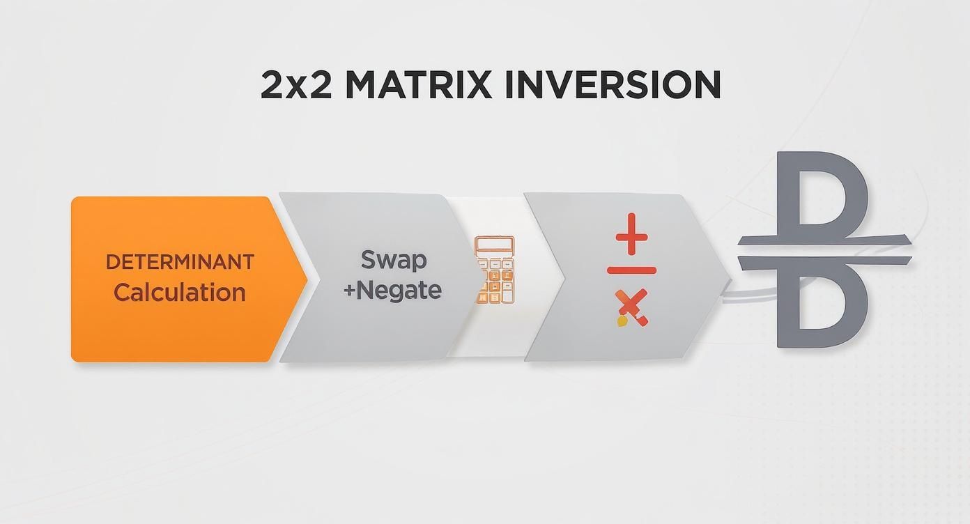
This flowchart neatly summarizes the quick, formulaic approach that simply isn't available for larger matrices.

A Worked Example: Inverting a 3x3 Matrix

Theory is great, but let's walk through an actual example. We'll find the inverse of matrix A:

A = [ 1 2 3 ]
[ 0 1 4 ]
[ 5 6 0 ]

We begin by setting up our augmented matrix with the 3x3 identity matrix next to it.

[ 1 2 3 | 1 0 0 ]
[ 0 1 4 | 0 1 0 ]
[ 5 6 0 | 0 0 1 ]

Now, we'll go column by column to turn the left side into [1 0 0], [0 1 0], and [0 0 1].

Tackling Column 1
Our target is to get the first column to look like [1, 0, 0]. The 1 at the top is already there—perfect! The 0 in the second row is also in place. All we need to do is eliminate the 5 in the third row. To do that, we'll replace Row 3 with Row 3 - 5 * Row 1.

[ 1 2 3 | 1 0 0 ]
[ 0 1 4 | 0 1 0 ]
[ 0 -4 -15 | -5 0 1 ]

Column 1 is done.

Moving on to Column 2
Next, we want the second column to be [0, 1, 0]. We already have the 1 in the middle, which is a great starting point. Now we need to create zeros above and below it.

• First, let's get rid of the 2 in the top row. We'll replace Row 1 with Row 1 - 2 * Row 2.
• Next, we'll eliminate the -4 in the bottom row by replacing Row 3 with Row 3 + 4 * Row 2.

After those two operations, our matrix looks like this:

[ 1 0 -5 | 1 -2 0 ]
[ 0 1 4 | 0 1 0 ]
[ 0 0 1 | -5 4 1 ]

Excellent. Two columns down, one to go.

Finishing with Column 3
The last goal is to make the third column [0, 0, 1]. Hey, look at that—the 1 at the bottom is already there! Now we just need to zero out the numbers above it.

• To handle the -5 in the top row, we'll do Row 1 + 5 * Row 3.
• To handle the 4 in the middle row, we'll do Row 2 - 4 * Row 3.

This brings us to our final form:

[ 1 0 0 | -24 18 5 ]
[ 0 1 0 | 20 -15 -4 ]
[ 0 0 1 | -5 4 1 ]

The left side is now the identity matrix, which means the matrix on the right is our answer. We've found A⁻¹!

An Expert Tip: The single biggest point of failure in this method is simple arithmetic. I've seen it happen countless times. You make one tiny calculation error in an early step, and it cascades, throwing the entire result off. Always, always double-check your row operations as you go. It’s far less painful than having to start from scratch.

Gauss-Jordan is a powerful and reliable process. It might feel a bit tedious, but its logical, step-by-step nature makes it the best way to manually find the inverse of any larger matrix.

Finding the Inverse with the Adjugate Matrix Method

While the Gauss-Jordan method is a reliable workhorse, there's another powerful approach that ties the inverse directly to the determinant. This is the adjugate matrix method, and it all comes down to one elegant formula:

A⁻¹ = (1/det(A)) * adj(A)

In plain English, this says the inverse is simply the adjugate of the matrix (adj(A)) multiplied by one over the determinant. This might seem more abstract than row reduction, but it can be a much faster route, especially if you've already found the determinant for another reason. You're already halfway there!

This method has deep historical roots. It was Arthur Cayley, in his foundational 1858 paper 'Memoir on the Theory of Matrices', who first clearly described how to construct a matrix inverse using its determinant. This provided a systematic approach that we still learn today. You can dig into the history of matrix theory to see just how these core ideas came to be.

What Goes Into the Formula?

To make this method work, you need to understand its three main ingredients: the determinant, the cofactor matrix, and finally, the adjugate matrix.

1. Calculate the Determinant (det(A)): This is your first gate. If the determinant is zero, stop right there. The matrix is singular, and no inverse exists.
2. Build the Matrix of Cofactors: This is where most of the work happens. For every single element in your original matrix, you'll calculate a corresponding "cofactor."
3. Find the Adjugate Matrix (adj(A)): This last piece is surprisingly easy. The adjugate is just the transpose of the cofactor matrix you built in the previous step.

Once you have these parts, you just assemble them according to the formula. Let's break down how to get that cofactor matrix.

Calculating Minors and Cofactors

The road to the adjugate begins with finding the "minor" for each element in your original matrix. A minor is just the determinant of the smaller matrix you get when you delete the row and column of the element you're looking at.

From the minor, you get the cofactor. This is where you have to pay attention to a "checkerboard" pattern of signs. You multiply the minor by either +1 or -1 based on its position in the matrix.

For a 3x3 matrix, the sign pattern looks like this:
[ + - + ]
[ - + - ]
[ + - + ]

So, a cofactor is really just a "signed minor."

A classic trip-up here is forgetting the sign pattern. It's so easy to meticulously calculate all the minors correctly but then forget to flip the signs where needed. This one small mistake will throw off the entire cofactor matrix and the final answer.

A 3x3 Example From Start to Finish

Let's use this method to find the inverse of the same matrix A from our Gauss-Jordan example:

A = [ 1 2 3 ]
[ 0 1 4 ]
[ 5 6 0 ]

First, the Determinant

Using the standard expansion method for a 3x3 determinant, we get:
det(A) = 1(10 - 46) - 2(00 - 45) + 3(06 - 15)
det(A) = 1(-24) - 2(-20) + 3(-5) = -24 + 40 - 15 = 1

The determinant is 1, which is not zero, so we're clear to proceed. An inverse definitely exists.

Next, the Matrix of Cofactors

Now for the main event. We have to calculate the cofactor for all nine positions. For instance, to get the cofactor for the top-left '1', we cross out its row and column, find the determinant of the remaining 2x2 matrix [1 4; 6 0], which is -24, and apply the positive sign from the checkerboard. We do this for every element.

After repeating this process for all nine spots, we end up with our full matrix of cofactors:

C = [ -24 20 -5 ]
[ 18 -15 4 ]
[ 5 -4 1 ]

Then, Find the Adjugate

This is the easy part. To get the adjugate, adj(A), we just transpose the cofactor matrix C. Rows become columns, and columns become rows.

adj(A) = Cᵀ = [ -24 18 5 ]
[ 20 -15 -4 ]
[ -5 4 1 ]

Finally, Calculate the Inverse

We're ready to plug everything into our formula: A⁻¹ = (1/det(A)) * adj(A).
Since our determinant is 1, the final calculation is trivial:

A⁻¹ = (1/1) * [ -24 18 5 ] = [ -24 18 5 ]
[ 20 -15 -4 ] [ 20 -15 -4 ]
[ -5 4 1 ] [ -5 4 1 ]

And there it is—the exact same result we found using Gauss-Jordan elimination. While the adjugate method can feel a bit more formulaic, it’s a powerful and historically important tool for finding an inverse.

Where Matrix Inverses Are Used in the Real World

https://www.youtube.com/embed/KoKWMSABkuM

Learning to find the inverse of a matrix can feel pretty abstract at first. But trust me, this isn't just a math exercise for a final exam. It's the engine running behind the scenes in technologies and scientific models that shape our world. Matrix inversion is a powerful tool for solving very real problems.

The most direct application you'll encounter is solving systems of linear equations. Any system can be boiled down to a clean, simple equation: Ax = b. Here, A is the matrix holding the coefficients, x is the vector of your unknown variables, and b is the vector of constants.

Instead of wrestling with substitution or elimination, you can find the solution in one fell swoop if A has an inverse: x = A⁻¹b. By multiplying both sides by the inverse of A, you instantly isolate the variables and solve for everything at once. This isn't just a neater trick; for massive systems, it's a cornerstone of computational mathematics.

Transforming Our Digital World

Beyond basic equations, matrix inverses are fundamental to computer graphics. Every time you watch a character sprint across a video game screen or rotate an object in a 3D modeling program, you're witnessing matrix operations at work.

• Rotation, Scaling, and Translation: Each of these movements is represented by a specific matrix. To undo that action—like returning a character to its starting position—you just multiply by the inverse of the transformation matrix.
• Camera Positioning: In 3D graphics, the "camera" or viewpoint is also controlled by matrices. The inverse is crucial for figuring out how objects should appear from that specific perspective, a vital step in rendering any scene.

This ability to reverse operations is what makes dynamic, interactive digital worlds feel so fluid. Without inverse matrices, every animation would be a one-way trip.

Securing Information and Modeling Economies

The applications don't stop there. In cryptography, matrices are used to encrypt messages. A message is converted into a matrix of numbers and then multiplied by a secret "encoding matrix."

The only way to decrypt the scrambled message is for the recipient to multiply it by the inverse of that encoding matrix. Doing so restores the original, readable text.

Economists also rely heavily on matrix inversion for input-output models. These models map out how the output of one industry (like steel) serves as the input for another (like automotive). The inverse of the model's "technology matrix" lets economists calculate the total output needed from every single sector to satisfy a given consumer demand.

Practical Pitfalls and How to Avoid Them

As powerful as finding an inverse can be, the process is incredibly sensitive. A single mistake can throw off the entire calculation.

My Experience: The most common error I see students make isn't conceptual; it's a simple arithmetic slip. During a long Gauss-Jordan elimination, miscalculating one value in a row operation can cascade, leading to a completely wrong answer that's frustrating to track down.

Here are the most frequent mistakes to watch out for:

• Sign Errors: Forgetting the "checkerboard" pattern of signs when finding cofactors for the adjugate method is a classic mistake.
• Arithmetic Mistakes: Tiny addition or multiplication errors during row reduction are incredibly common but have disastrous results.
• Incorrect Swaps: When using the 2x2 shortcut, it's easy to accidentally negate the main diagonal elements instead of swapping them, especially under pressure.

The absolute best way to catch these slips is to verify your work. Once you think you've found the inverse, A⁻¹, multiply it by your original matrix, A. If the result is the identity matrix, you can be confident your answer is correct. This final check takes a minute but can save you a world of hurt.

Using Tech to Find a Matrix Inverse Instantly

Learning to find an inverse by hand is crucial for really getting the concepts. It builds your intuition. But let's be honest—in the real world, nobody is doing Gauss-Jordan elimination on a 50x50 matrix with a pencil and paper. That’s where technology steps in.

For any problem bigger than a 3x3, or when you just need a fast, accurate answer without the risk of a calculation error, software is the way to go. It frees you up to think about what the numbers actually mean instead of getting lost in the arithmetic.

Python and NumPy for Heavy Lifting

If you're doing anything in data science, engineering, or scientific research, Python's NumPy library is your best friend for matrix math. Finding an inverse is a one-liner. Seriously.

You just use the np.linalg.inv() command.

Here's a quick look from the official NumPy docs that shows how clean it is:

The code sets up a matrix a, then calculates its inverse ainv in a single step. The final check, multiplying a by ainv, gives the identity matrix, proving it worked perfectly. It's that simple.

Quick Checks with a Graphing Calculator

For students, a graphing calculator like the TI-84 is a lifesaver for checking homework or solving problems in a pinch. The process is incredibly straightforward.

• First, head to the matrix editor on your calculator.
• Next, define the size (e.g., 3x3) and punch in the elements of your matrix.
• Then, go back to the home screen, select your matrix by name (like [A]), and hit the inverse key (x⁻¹).
• Press enter, and boom—the inverse appears.

This is a fantastic way to double-check your work after slogging through the adjugate method or row reduction. For more complex problems where you want to see the steps broken down, you might also find that an AI math solver can offer detailed guidance.

The Bottom Line: Knowing how to find an inverse by hand builds a solid foundation. But for real-world efficiency and accuracy, you need to be comfortable with technology. Use calculators and code libraries to verify your answers and tackle the big, messy problems that are impractical to solve manually.

Common Questions and Sticking Points with Matrix Inverses

Even after you've got the methods down, a few questions always seem to pop up when you're wrestling with matrix inverses. That's perfectly normal—some of these concepts are genuinely tricky. Let's walk through a few of the most common hangups to build your confidence.

One of the first things people wonder is, why do only square matrices have an inverse? Why not rectangular ones? It all comes back to what an inverse is actually for: it’s meant to perfectly "undo" a linear transformation.

A square matrix (like a 2x2 or 3x3) takes a vector from a space and maps it to a new vector in the same space. Think of it as transforming a 2D plane into another 2D plane. But a rectangular matrix changes the dimensions. It might take a 2D vector and map it into 3D space. You just can't reverse that kind of dimensional jump with a single matrix multiplication, which is why the whole idea of an inverse is reserved for square matrices only.

What Does a Zero Determinant Really Mean?

This is a big one. You learn the rule: if the determinant is zero, there's no inverse. But why?

Imagine a matrix as a machine that transforms space. A matrix with a determinant of zero is a machine that crushes everything flat. A 2x2 matrix with a zero determinant might take an entire 2D plane and squash it down onto a single line. When you do that, you lose a whole dimension's worth of information. There's simply no way to reverse the process and get back to the original plane.

That irreversible collapse is the core reason why a zero determinant signals that no inverse exists.

An inverse matrix guarantees a single, unique solution. A zero determinant means you've got either no solution or infinitely many solutions for a related system of equations, which breaks the one-to-one mapping an inverse requires.

Which Method is the "Best"?

Finally, students often ask if there's one superior method for finding an inverse. The honest answer is: it depends entirely on the matrix you're dealing with.

• For any 2x2 matrix: The shortcut formula is a no-brainer. It's the fastest and most direct way every single time.
• For 3x3 or larger (by hand): I usually find Gauss-Jordan elimination is more reliable. While the adjugate method can feel more formulaic, it’s also easy to make a small sign error with all the cofactors. Row reduction is more systematic, though the arithmetic can be tedious.
• When using a computer: This is where it gets interesting. Explicitly telling software to calculate inv(A)*b is often less efficient and numerically less stable than just asking it to solve the system A\b. That's because programs like Python with NumPy use highly optimized algorithms (like LU decomposition) that find the solution without ever computing the full inverse.

Knowing these little details helps you pick the right tool for the job and understand what's happening behind the scenes.

---

Feeling stuck on a tough matrix problem or any other homework? Feen AI can help. Upload a picture of your problem, and our AI-powered tutor will provide clear, step-by-step explanations to guide you to the answer. Get unstuck and study smarter.