How to Graph Linear Inequalities A Practical Guide

When you first look at a linear inequality, it might seem tricky to graph. But the truth is, if you can graph a straight line, you're already 90% of the way there. We just need to add two more layers: deciding what kind of line to draw and figuring out which side to shade.

It boils down to a simple, repeatable process: format, draw, and shade. That's the whole game. Once you get this rhythm down, you can tackle any linear inequality that comes your way.

Your Starting Point for Graphing Linear Inequalities

Before we get into the nitty-gritty of slope-intercept form and test points, let's zoom out and look at the big picture. The goal here isn't to memorize rules but to understand the logic. Every linear inequality graph follows the same fundamental workflow.

This visual gives you a quick snapshot of the entire process, from getting the inequality ready to finding the final solution.

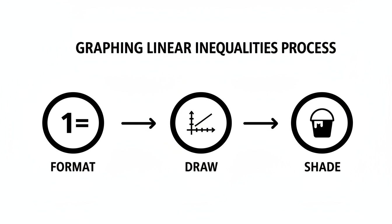
Think of these as building blocks. Each step logically follows the one before it, leading you straight to an accurate graph that shows every possible solution.

To make this crystal clear, let's break down the process into three core phases. The table below outlines what you need to do and, just as importantly, why you're doing it.

The Three Core Phases of Graphing a Linear Inequality

Phase	Action Required	Key Decision
1. Format	Temporarily treat the inequality as a standard linear equation (e.g., y = mx + b).	This isolates the equation for your boundary line, making it easy to graph.
2. Draw	Plot the boundary line on the coordinate plane using its slope and y-intercept.	Decide if the line is solid (≤ or ≥) or dashed (< or >).
3. Shade	Pick a test point (like (0,0)) to see which side of the line satisfies the original inequality.	Shade the entire region that represents the "true" side of the line.

This framework takes the guesswork out of the process. You're not just randomly drawing and shading; you're making intentional decisions at each stage to define the solution.

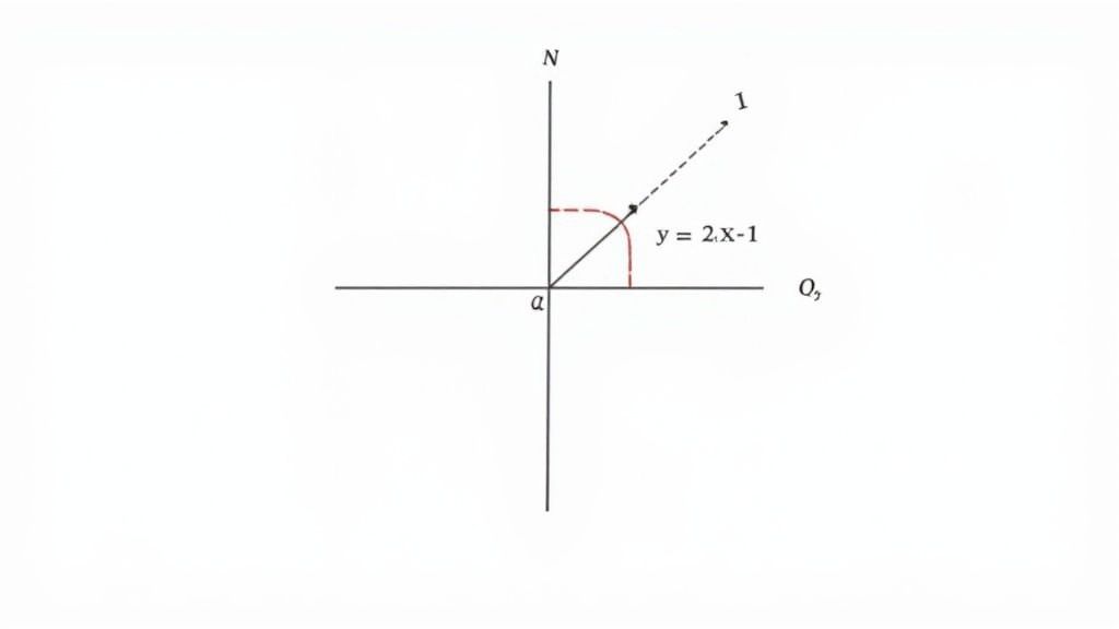
Let’s walk through this with a quick example, say y > 2x - 1.

First, you'd zero in on the equation part, y = 2x - 1. This is what you'll actually plot on the graph. It acts as a fence, separating the coordinate plane into two distinct halves.

Next, you draw that line. We'll get into the "solid vs. dashed" rules in a moment, but for now, just picture the line y = 2x - 1 cutting across your graph. This is your boundary.

Finally, you figure out which side of the fence contains all the answers. You'll shade one entire side of the line, creating a visual representation of the infinite coordinate pairs that make the original inequality, y > 2x - 1, true.

The solution to a linear inequality isn't a single point or a line; it's an entire region of the graph. Your job is to correctly identify and shade this specific "solution space."

This core idea of a solution space is a huge concept in math. While we're focusing on lines here, the principle of defining boundaries applies to all sorts of functions. For a deeper dive into how these boundaries work, you can explore our guide on how to find the domain and range of a function.

Solid or Dashed? Drawing the Boundary Line

Once you've got your inequality in slope-intercept form, it's time to put pencil to paper and draw the boundary line. But hold on—this isn't just about connecting the dots. How you draw this line is a crucial piece of the puzzle.

Getting this part wrong is one of the most common slip-ups I see. The good news is that the inequality symbol itself gives you a very clear instruction on what to do. You just have to know how to read it.

The Solid Line: An Inclusive Boundary

Think of a solid line as a solid wall. It means that any point sitting directly on that line is part of the solution. This happens when your inequality includes the possibility of being "equal to" the line.

• You'll draw a solid line for inequalities with ≥ (greater than or equal to) and ≤ (less than or equal to).
• For example, with the inequality y ≤ -x + 3, any coordinate pair that falls perfectly on the line y = -x + 3 is a totally valid solution.

The Dashed Line: An Exclusive Boundary

On the flip side, a dashed line acts more like an open doorway or a dotted line on a map. It marks the edge of the solution area, but the points on the line itself aren't included. This is for inequalities that are strictly "greater than" or "less than."

• You'll draw a dashed line for inequalities with > (greater than) and < (less than).
• For an inequality like y > -x + 3, a point sitting right on the line y = -x + 3 doesn't actually work as a solution. The dashed line is our visual cue for this exclusion.

This whole idea of graphically defining solution sets isn't new. The foundational concepts were being hammered out in the late 19th century with work like the Minkowski–Farkas theorem, which gave us a more formal way to understand these boundaries. If you're a history buff, you can explore more about the evolution of linear inequalities on Encyclopedia of Math.

My Favorite Tip: Look for the little "or equal to" bar in the ≤ or ≥ symbols. That extra horizontal line is your reminder to draw a solid line on your graph. No bar, no solid line!

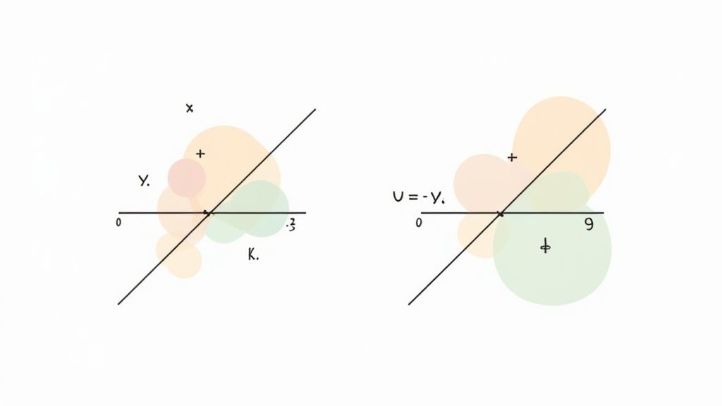
Let's look at two inequalities side-by-side. They share the same boundary equation, y = 2x - 1, but that tiny difference in the inequality symbol changes the graph.

Inequality	Boundary Line	What it Really Means
y ≥ 2x - 1	Solid	Any point on the line y = 2x - 1 is a solution.
y > 2x - 1	Dashed	Points on the line y = 2x - 1 are not solutions. Only the points in the shaded region are.

Nailing this distinction is essential for making sure your graph tells the whole story. It’s a small detail with a big impact. Now that we have the boundary line drawn correctly, let's figure out which side to shade.

Figuring Out Where to Shade: The Test Point Method

Okay, you've got your boundary line on the graph—solid or dashed, depending on the inequality. Now the graph is split in two. The final piece of the puzzle is deciding which side to shade. You could guess and have a 50/50 shot, but there’s a foolproof way to get it right every single time: the test point method.

It's a simple idea. You just pick one point on the graph—any point not on the line—and plug its coordinates into the original inequality. If the numbers work out and the statement is true, you've found your solution zone.

Why the Origin Is Your Go-To Test Point

In most cases, the absolute easiest point to work with is the origin: (0, 0). Why? Because plugging zeros into an inequality makes the math dead simple. You can usually do it in your head.

The only time you can't use (0, 0) is when the boundary line runs straight through it.

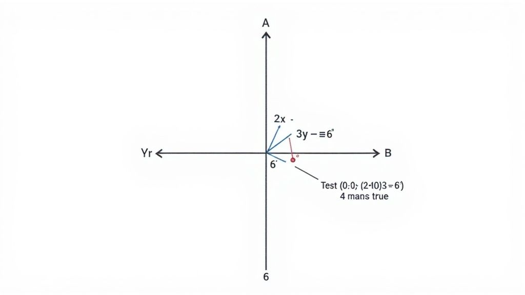
Let's see how this works with our inequality 2x + 3y < 6.

First, check if (0, 0) is a valid test point. The line 2x + 3y = 6 doesn't pass through the origin, so we're good to go.

Now, substitute the point into the inequality: 2(0) + 3(0) < 6.

This simplifies down to 0 < 6. Is that true? Absolutely.

Since our test point (0, 0) created a true statement, we know it's part of the solution. So, we shade the entire region on the same side of the line as the origin.

Key Takeaway: If your test point makes the inequality true, shade the region that includes that point. If it makes the inequality false, shade the other side.

This simple idea of finding solution regions is the backbone of a powerful field called linear programming. It exploded in use after World War II, when the "simplex method" was developed in 1947. Suddenly, graphing inequalities became a practical tool for optimization. By 1952, it was being used to manage around 80% of U.S. military logistics, saving what would be $20 billion in today's money. You can learn more about the rise of linear programming on YouTube.

What to Do When the Line Crosses the Origin

Sooner or later, you'll get an inequality where the boundary line slices right through (0, 0), like y ≥ -4x or 2x - y > 0. When that happens, you just have to pick a different point. Any point will do, as long as it isn't on the line.

I usually go for something simple like (1, 1), (0, 1), or (1, 0).

Let's try this with the inequality y > 2x.

• The boundary line y = 2x goes through the origin, so (0, 0) is out.
• Let's pick (0, 3) as our new test point. It's easy to see it's not on the line.
• Plug it into the inequality: 3 > 2(0).
• This simplifies to 3 > 0, which is true.

Since our point (0, 3) worked, we just shade the entire half of the graph where (0, 3) is located. Once you get the hang of the test point method, you'll be able to graph any linear inequality with confidence, no matter where the line ends up.

Graphing Systems of Linear Inequalities

If you’ve got a handle on graphing a single linear inequality, you’re already most of the way there. Tackling a system of inequalities is less of a leap and more of a small step. The core idea is that you're no longer looking for one shaded area, but for the overlap between all the shaded areas. This overlapping zone is the sweet spot on the graph where every single inequality in the system is true.

I like to think of it as two different colored highlighters. You shade the solution for the first inequality in yellow and the solution for the second in blue. The "solution" to the system is wherever the two colors mix to make green. Your mission is to find that green region.

A Step-By-Step Walkthrough of Graphing a System

Let’s get our hands dirty with a classic example. We'll graph the system containing x + y ≥ 3 and y < 2x - 1.

The trick is to focus on one inequality at a time. Just pretend the other one doesn't exist for a moment.

First up: x + y ≥ 3

• First thing's first, let's get it into slope-intercept form: y ≥ -x + 3.
• The boundary line is y = -x + 3. The ≥ symbol tells us this will be a solid line.
• Let’s use our trusty (0, 0) test point. Plugging it in gives us 0 ≥ -0 + 3, which simplifies to 0 ≥ 3. That’s definitely false.
• Because our test point failed, we shade the side of the line that doesn't include the origin.

Next, let's handle y < 2x - 1

• This one is already in slope-intercept form, which saves us a step.
• Our boundary line is y = 2x - 1. The < symbol means we need a dashed line this time.
• Checking the (0, 0) point again, we get 0 < 2(0) - 1, or 0 < -1. This is also false.
• So, we'll shade the side of this dashed line that doesn't contain the origin.

Once you’ve graphed both, you'll see two different shaded regions on your coordinate plane. The real solution to the system is the one specific area where those two regions cross over each other.

Pro Tip: When you're sketching these by hand, it’s a huge help to use different shading patterns. Maybe use diagonal lines slanting one way for the first inequality and slanting the other way for the second. The part of your graph that ends up looking like a crosshatch or checkerboard is your answer.

This whole process of finding a common solution area is a fundamental concept in algebra. It’s the visual counterpart to the algebraic methods you'd use for equations, which you can see in our guide on how to solve systems of linear equations.

This quick reference table can help you interpret what you're seeing on the graph when you're working with a system of two inequalities.

Interpreting Shading for Systems of Inequalities

Scenario	Description	What the Solution Looks Like
Overlap Between	Both inequalities are "less than" or "less than or equal to".	The solution is typically the region below both boundary lines.
Overlap Above	Both inequalities are "greater than" or "greater than or equal to".	The solution is typically the region above both boundary lines.
Sandwiched Region	One inequality is "greater than" and the other is "less than".	The solution is the area between the two boundary lines.
No Overlap	The shaded regions point away from each other and never intersect.	There is no solution to the system.

Remember, this is a general guide. The exact location always depends on the specific slopes and y-intercepts of your lines, so always graph them carefully!

What About When There's No Solution?

Yes, it's totally possible for a system of inequalities to have no solution at all. This happens when the shaded regions simply never overlap.

Picture two parallel lines on a graph. If one inequality tells you to shade above the higher line, and the second tells you to shade below the lower line, their shaded zones will stretch out into infinity without ever meeting. When this happens, there isn't a single (x,y) point in the universe that can satisfy both conditions at the same time. The solution set is empty.

Common Mistakes and How to Sidestep Them

Graphing linear inequalities has a few moving parts, and it's easy to make a small mistake that throws the whole thing off. Knowing where most people trip up is half the battle. Think of it as knowing where the potholes are before you start driving.

One of the most common errors happens right at the beginning, before you even put pencil to paper. It’s all about what you do when a negative number gets involved in your algebra.

The Dreaded Sign Flip

Let’s imagine you're faced with an inequality like -2y > 4x - 6. Your first instinct is to isolate y to get it into that familiar slope-intercept form. To do that, you have to divide everything by -2.

This is the moment of truth. Whenever you multiply or divide both sides of an inequality by a negative number, you absolutely must flip the inequality sign. It's a non-negotiable rule.

Forget this step, and your inequality mistakenly becomes y > -2x + 3. The correct answer is actually y < -2x + 3. That one tiny symbol flips the entire meaning of the graph, causing you to shade the wrong half of the plane. It's a simple rule, but it's so easy to miss when you're moving fast.

My Personal Tip: After I isolate y, I literally circle the inequality sign with my pencil. Then I look back at my work. Did I divide by a negative? If so, I double-check that the circled sign is pointing the opposite way from where it started. This little habit has saved me countless times.

Mixing Up Shading Directions

The other major pitfall is shading the wrong region. You do all the hard work—you find the boundary line, you pick a great test point like (0,0), and you plug it in. The test comes back false... but in your haste, you shade the region containing the origin anyway. It happens to the best of us.

Here’s a simple system to prevent that. If your test point gives you a false statement, immediately draw a small "X" on that point. That’s your signal to shade the other side. If the statement is true, draw a checkmark and shade the region containing that point. This creates a quick visual cue that keeps you on track.

Along those same lines, be cautious with the "above/below" shortcut. The trick of shading above the line for y > and below for y < is fantastic, but it only works once you've solved the inequality for y.

This is a common trap with inequalities given in standard form, like 3x - y < 5. You can't just look at that less-than sign and assume you're shading below the line. You have to isolate y first! Word problems often present information in a similar format, so it's a good skill to master. If you're looking for more on that, check out our guide on how to solve word problems in algebra.

Common Questions About Graphing Inequalities

Once you get comfortable with the basic steps for graphing linear inequalities, you'll inevitably run into some oddball problems. Let's tackle some of the most common "what if" scenarios that trip students up.

What if an Inequality Only Has One Variable?

It can be a little jarring to see something like x > 3 or y ≤ -2. Where did the y = mx + b form go? Don't worry, these are actually the easiest types to graph. They just represent straight vertical or horizontal lines.

Take x > 3. First, just think about the equation x = 3. That's simply a vertical line that passes through the number 3 on the x-axis. Since our inequality symbol is ">" (greater than), the line itself isn't part of the solution, so we draw a dashed vertical line. Now for the shading: where are all the x-values bigger than 3? That's everything to the right of the line. Shade that whole side.

It works the same way for y ≤ -2. Start with the horizontal line y = -2. Because the symbol is "≤" (less than or equal to), this line will be solid. Then, just shade where the y-values are less than -2—which is everything below the line.

Is There a Shortcut for Shading?

Yes, and it's a popular one, but you have to be careful. This trick only works when the inequality is in slope-intercept form, with y isolated on the left side.

Here’s the shortcut:

• For y > or y ≥, you shade above the boundary line.
• For y < or y ≤, you shade below the boundary line.

This can definitely save you a moment, but it’s easy to mess up. If you try to use this shortcut on an inequality like 3x - 2y < 8 before solving for y, you'll almost certainly shade the wrong region. My advice? Stick with the test point method. It’s foolproof and works every time, which makes it a much safer bet, especially when you're just starting out.

Can a System of Inequalities Have No Solution?

Absolutely. It’s totally possible for the shaded regions of a system of inequalities to never overlap. When that happens, there's no single point on the entire coordinate plane that satisfies all the inequalities.

A classic example of a no-solution system involves parallel lines. Imagine you need to graph y > x + 4 and y < x - 1. Both lines have the same slope, so they'll run alongside each other forever and never intersect. The first inequality tells you to shade above the top line, while the second tells you to shade below the bottom line. Their solution regions will never meet in the middle.

In cases like this, the answer is simply "no solution." There isn't a single (x, y) coordinate pair that can make both inequalities true at the same time.

For a broader look at teaching methods, you can also explore some strategies to motivate high school students with technology.

---

Hitting a wall with a tough inequality or another homework problem? Feen AI can get you unstuck. Just snap a photo of your problem, and our AI tutor will walk you through it with clear, step-by-step explanations. It’s all about understanding the concept, not just copying an answer. Give it a try at https://feen.ai and see how much easier homework can be.